PCA Spike Sorting
Common Use Cases

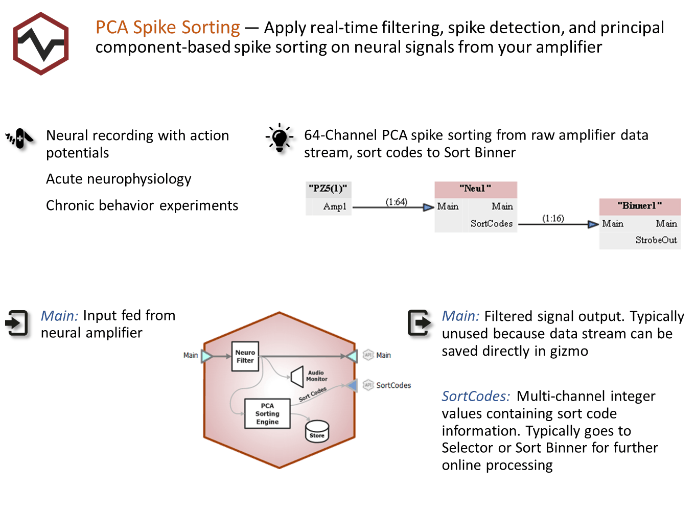
Real-time filtering, spike detection, and principal component-based spike sorting with selectable algorithms. This is the most common method for online spike sorting. Cluster units in PCA space and identify spikes automatically or manually cut.
Gizmo Help Slides
Reference
The PCA Spike Sorting gizmo performs filtering, thresholding and online principal component-based spike sorting and storage on multi-channel neural signals at sampling rates up to 50 kHz (up to 100 kHz for very low channel count).
Data Storage
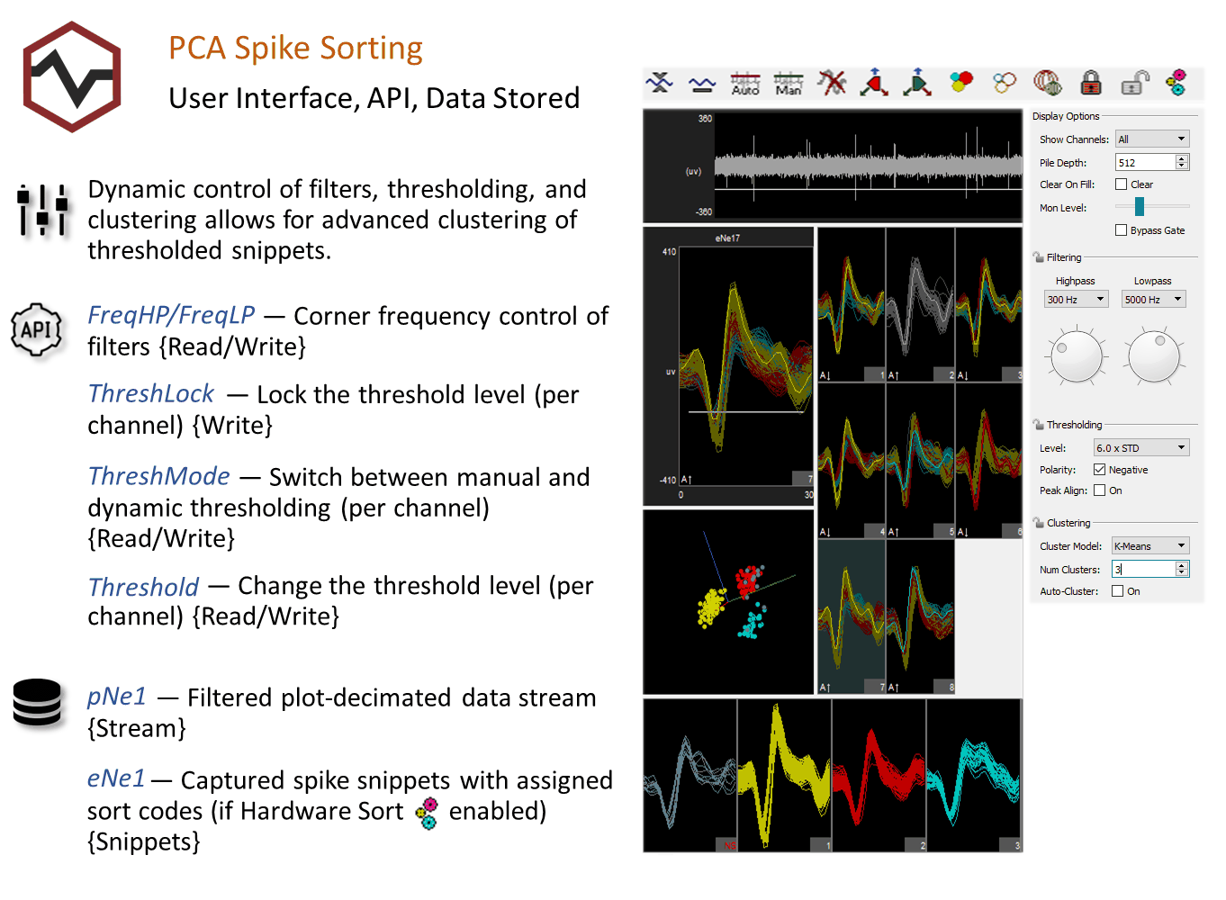
This gizmo generates two types of data for storage: snippet data (includes timestamp, short waveform, and sort code) and plot decimated data streams. The stream data generated by this gizmo is a highly decimated version of the waveforms that keeps local maximum and minimum values of the filtered signals, which makes it ideal for visualizing high frequency spike activity on a computer monitor with a fixed number of pixels.
In plots and in the data tank, each type of data is designated with a prefix: 'e' for snippets and 'p' for streams. You can opt to save only snippets or to disable storage in the gizmo's configuration settings. The sort codes can be configured as an output to be used in other gizmos.
Threshold Detection
At runtime, candidate spikes are detected based on a calculation of the deviation of a waveform from its RMS. By default, the timestamp and position of the waveform in the snippet is dependent on the time of the threshold crossing for the signal. An alternative setting allows waveform timestamp and positioning to be determined by the waveform's highest peak, aligning snippets to their respective peaks. By default, detection is automated and you can make adjustments in the threshold control plot in the runtime window.
Spike Sorting
The sorting interface works in three phases:
-
Training
-
Classification
-
Sorting
Training
During an initial training period, candidate waveforms are collected and used to compute the first three principal components with the largest possible variance for each recording channel. Incoming waveforms are transformed and appears as dots in the three-dimensional feature space.
Classification
Dots in the feature space are then clustered to isolate waveforms that were recorded from the same neuron. By default, auto-clustering is disabled and no clustering (or sorting) takes place until it's initiated. The default clustering method is a Bayesian algorithm, but you can choose a K-Means method or use manual cluster cutting techniques. Preliminary identification of units is indicated by color coding in the plots provided for visualization; however, all candidate spikes are saved to the data tank with a sort code of 0 during this phase. During this phase you can explore the data and modify sort parameters without affecting saved data.
Sorting

When you're satisfied with the clustering, you can apply Hardware Sorts. The clustering parameters are sent to the hardware and sort codes will be applied to new data as it is acquired in real-time. This toolbar button must be 'pressed' for online sorting to take place on the hardware.
The Runtime Interface
Runtime Plot
Streamed waveform and snippet plots are added to the runtime window for visualization
PCA Spike Sorting Window
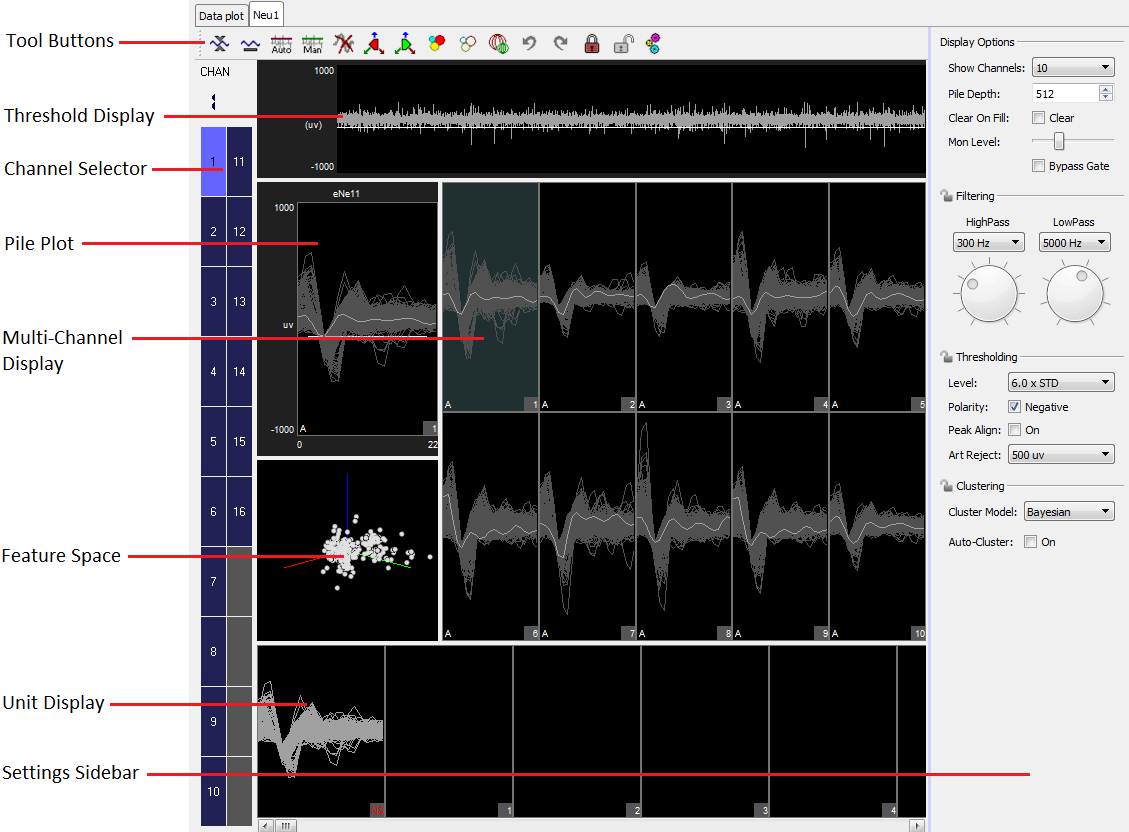
The runtime window includes:
Simple Zoom
You can zoom any plot to see more or less detail without affecting the actual data.
To change the zoom level, hold down the Shift key and left-click-drag the mouse up or down.
To reset the zoom level, hold down the Shift key and double-click the mouse within the display area.
Display Scale
To make it easier to see waveform shapes for channels with lower magnitude, you can scale individual channels manually or normalize all channels to fit to a similar scale, all without altering the data being stored.

To normalize all channels, click the Auto Scale button in the toolbar and choose to normalize the display. Each channel is scaled individually to fit around 80% of the signal's vertical size in each plot. An up or down arrow is displayed in the bottom left corner of the plot or subplot to indicate whether the display has been scaled up or down. This does not change the scale of the feature space.
To adjust the scale of a single channel, press and hold down the Ctrl key, and click-and-drag the mouse up or down in the Multi-Channel Display. While adjusting the display scale, the numeric value in the lower right corner of the channel plot indicates the new scale value.

To reset the scale for all channels, click the Reset Base Scale button. This does not remove any Zoom applied to a plot.
To return a single channel to its base scale, right-click the desired channel and select Reset Scaling from the menu.
Settings Sidebar
Threshold Control

Click the Auto Threshold button to initiate automatic threshold tracking on all unlocked channels. If auto thresholding is enabled in the designtime interface, real-time tracking will begin on all channels, otherwise the channels will remain in manual threshold mode and the threshold will be set based on a one-time calculation using the current window data and the Thresholding Level and Polarity settings.

Click the Manual Threshold button to enable manual thresholding on all unlocked channels. In manual threshold mode, the threshold bar may be adjusted by clicking and dragging the white bar in the threshold display window (shown below) or in the pile plot.
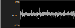 |
| Threshold Display in Manual Mode |
You can also right-click the plot at the desired threshold location and choose Set Threshold Here from the menu to move the threshold to that location on one channel. You have the option to apply this new location to all channels in manual thresholding mode.
Right-click the pile plot or threshold display and use the Auto/Manual Threshold options to change the threshold mode of an individual channel.
Feature Space
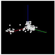 |
| Feature Space |
Viewing Events in the Feature Space
Click-and-drag in the feature space to rotate the view.
Press and hold the Alt key on the keyboard and click-and-drag to pan the feature space.
Press and hold the Shift key on the keyboard and double-click anywhere in the feature space to reset the feature space view.
Training
During training, as events are added to the display they become part of the data set used for feature space calculation. The feature space for each channel is periodically recalculated using all data in the history at that time, until the training is complete. Training ends when either the required number of events is reached or the training time period expires.
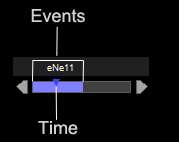 |
| Training Bar |
During the training period, a colored progress bar (shown above) is added to all pile plots to show how many events are required, or how much time has elapsed. By default, the progress bar is colored blue. If Auto-Cluster is enabled in the settings sidebar, the progress bar is red.
Arrows located on either end of the training progress bar can be used to restart the training period (left arrow) or to accept the current feature space (right arrow) for the active channel.

Click the Accept Current Space button to accept the current feature space for all channels. Accept the feature space on individual channels by right- clicking on any plot of an actively training channel and selecting Accept Space.

Training on all channel can be initiated by clicking the Recalculate Space button. Training can be initiated on individual channels by right-clicking any plot and selecting Recalculate Space.
Using Clusters for Classification

Click the Cluster Automatically button to calculate clusters for all channels using the options in the settings sidebar. If training is active, this stops training and accepts the feature space before clustering. Each waveform identified by a sort code is represented by a single color on all plots. To cluster an individual channel, right-click on the pile plot or threshold display and choose Auto Cluster.
Click the Clear Clusters button to remove all clusters on unlocked channels. To clear clusters from an individual channel, right-click on the channel plot and choose Clear Clusters. Sort codes already saved to disk remain unchanged.
Click the Show Spheres button to view the boundaries of spheres used to define cluster shapes in the feature space.
Applying Sorts to New Data
Sort codes are not saved to the data tank until you apply sorts. You can re-sort or make adjustments as needed to get the best results.
Click the Hardware Sort button to send the sorting parameters to the hardware and begin saving sort codes to the data tank. Sort codes are applied as new data is acquired. While this button is down, any changes in sorting parameters in the display will be sent to the hardware and applied automatically to new data.
Locking Channels

Click the Lock All button to lock the clusters for all channels, or right- click individual channels and choose Lock . If training is active, locking any channel also ends any the training and accepts the feature space.

Click the Unlock button to unlock all channels, or right-click individual channel plots and choose Unlock.
The Unit Display
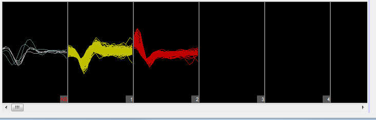 |
| Unit Display |
In the Unit Display, candidate waveforms from the currently selected channel are grouped by sort code. Unsorted (sort code 0) and outlier (sort code 31) waveforms are displayed to the left with the label NS.
The maximum number of sort codes (up to five) that can be sorted on the hardware is determined by the Max Clusters (Sort Codes) configuration setting. Assigned sort codes larger than this value are displayed in red to indicate they are only visible in the software interface. These waveforms will be given a sort code of 31 (outlier) in the data tank.
The Unit Display can be used to reassign units to different sort codes or combine two or more units together into a single unit by dragging the units.
PCA Spike Sorting Configuration Options
Sorting Tab
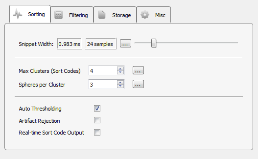 |
| Sorting Options Tab |
Snippet Width
Drag slider to select the desired width (displayed in milliseconds and samples) of recorded snippets.
Max Clusters (Sort Codes)
Events that contain similar characteristics are grouped into clusters and are given the same sort code. The maximum number of clusters supported in hardware sorting is five. Allowing a larger number of clusters increases processing overhead, but accommodates greater variability in the data set.
Spheres per Cluster
Spheres in the three-dimensional PCA feature space are used to define each cluster. The maximum number of spheres supported is five, per cluster per channel. Allowing a larger number of spheres to the sorting algorithm increases processing overhead, but provides a more accurate fit for a cluster's shape.
Auto Thresholding
In automatic thresholding, the threshold used to record snippets is adjusted in real-time to changes in each channel waveform's RMS. The previous five seconds of data are used in the RMS calculation.
Artifact Rejection
When artifact rejection is enabled, snippets that contain at least one sample greater than the artifact rejection level set on the runtime interface are ignored.
Real-time Sort Code Output
Make the multi-channel integer stream of compressed sort codes available to other gizmos, such as Sort Binner or UDP output.
Note: The sort code output is delayed by (window width + 2) samples from when the threshold is crossed. When artifact rejection is enabled, the sort code output is delayed by an additional window width, so (2 * window width + 2) total samples.
Filtering Tab
The gizmo applies a highpass and lowpass filter to all channels before spike detection. The runtime interface includes controls for dynamic adjustments to the filter settings. You also set default values in the Filtering Options tab.
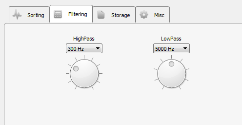 |
| Filtering Options Tab |
Storage Tab
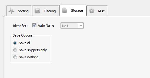 |
| Storage Options Tab |
Save Options
Select whether to save only snippet waveforms or to include the plot decimated waveforms used by the sorting gizmo or to save nothing at all to the data tank.
Misc Tab
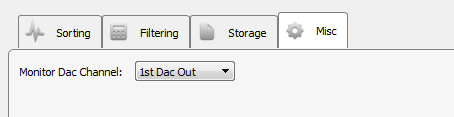 |
| Misc Options Tab |
Monitor DAC Channel
Select an output channel to send the monitor signal to, or set to Disable to turn monitoring off.