Stream Plot Example
Import continuous data into MATLAB using TDTbin2mat
Plot a single channel of data with various filtering schemes
Good for first-pass visualization of streamed data
Housekeeping
Clear workspace and close existing figures. Add SDK directories to MATLAB path.
close all; clear all; clc;
[MAINEXAMPLEPATH,name,ext] = fileparts(cd); % \TDTMatlabSDK\Examples
DATAPATH = fullfile(MAINEXAMPLEPATH, 'ExampleData'); % \TDTMatlabSDK\Examples\ExampleData
[SDKPATH,name,ext] = fileparts(MAINEXAMPLEPATH); % \TDTMatlabSDK
addpath(genpath(SDKPATH));
Importing the Data
This example assumes you downloaded our example data sets and extracted it into the \TDTMatlabSDK\Examples directory. To import your own data, replace 'BLOCKPATH' with the path to your own data block.
In Synapse, you can find the block path in the database. Go to Menu → History. Find your block, then Right-Click → Copy path to clipboard.
BLOCKPATH = fullfile(DATAPATH,'Algernon-180308-130351');
Now read channel 1 from all stream data into a MATLAB structure called 'data'.
data = TDTbin2mat(BLOCKPATH, 'TYPE', {'streams', 'epocs'}, 'CHANNEL', 1);
read from t=0.00s to t=61.23s
And that's it! Your data is now in MATLAB. The rest of the code is a simple plotting example.
Stream Store Plotting
Let's create time vectors for each stream store for plotting in time.
time_Wav1 = (1:length(data.streams.Wav1.data))/data.streams.Wav1.fs;
time_LFP1 = (1:length(data.streams.LFP1.data))/data.streams.LFP1.fs;
time_pNe1 = (1:length(data.streams.pNe1.data))/data.streams.pNe1.fs;
ax1 = subplot(3,1,1);
plot(time_Wav1, data.streams.Wav1.data(1,:)*1e6,'b');
axis tight;
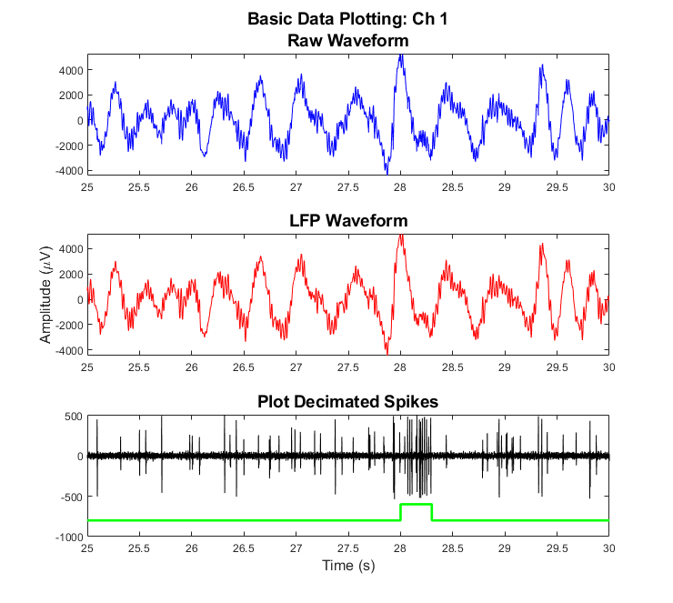
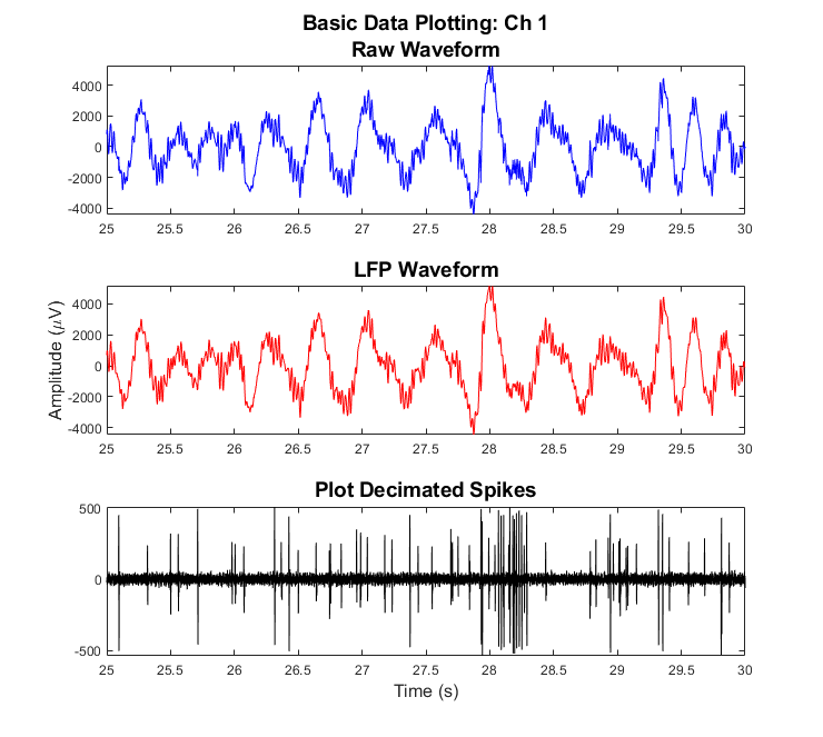
title({'Basic Data Plotting: Ch 1','Raw Waveform'},'FontSize',14)
xlim([25 30]);
ax2 = subplot(3,1,2);
plot(time_LFP1, data.streams.LFP1.data(1,:)*1e6,'r');
title('LFP Waveform','FontSize',14);
ax3 = subplot(3,1,3);
plot(time_pNe1, data.streams.pNe1.data(1,:),'k');
title('Plot Decimated Spikes','FontSize',14);
ax = [ax1, ax2, ax3];
axis([ax1 ax2], 'tight')
linkaxes(ax, 'x')
xlim(ax(end), [25 30]);
xlabel(ax(end), 'Time (s)','FontSize',12)
ylabel(ax(2), 'Amplitude (\muV)','FontSize',12);
% Enlarge figure.
set(gcf, 'Units', 'centimeters', 'OuterPosition', [10, 10, 20, 20]);
Epoc Events
Generate continuous time series for epoc data using epoc timestamps
% StimSync epoc event
STIMSYNC = 'PC0_';
pc0_on = data.epocs.(STIMSYNC).onset;
pc0_off = data.epocs.(STIMSYNC).offset;
pc0_x = reshape(kron([pc0_on, pc0_off], [1, 1])', [], 1);
Make a time series waveform of epoc values and plot them.
sz = length(pc0_on);
d = data.epocs.(STIMSYNC).data';
pc0_y = reshape([zeros(1, sz); d; d; zeros(1, sz)], 1, []);
hold on; plot(pc0_x, 200*(pc0_y) - 800, 'g', 'LineWidth', 2);