Licking Bout Epoc Filtering

This example looks at fiber photometry data in the VTA where subjects are provided sucrose water after a fasting period.
Lick events are captured as TTL pulses.
Objective is to combine many consecutive licking events into a single event based on time difference and lick count thresholds.
New lick bout events can then be used for clear peri-event filtering.

Download M File

Housekeeping

Clear workspace and close existing figures. Add SDK directories to MATLAB path.

close all; clear all; clc;

[MAINEXAMPLEPATH,name,ext] = fileparts(cd); % \TDTMatlabSDK\Examples
DATAPATH = fullfile(MAINEXAMPLEPATH, 'ExampleData'); % \TDTMatlabSDK\Examples\ExampleData
[SDKPATH,name,ext] = fileparts(MAINEXAMPLEPATH); % \TDTMatlabSDK
addpath(genpath(SDKPATH));

Importing the Data

This example assumes you downloaded our example data sets and extracted it into the \TDTMatlabSDK\Examples directory. To import your own data, replace 'BLOCKPATH' with the path to your own data block.

In Synapse, you can find the block path in the database. Go to Menu → History. Find your block, then Right-Click → Copy path to clipboard.

BLOCKPATH = fullfile(DATAPATH,'VTA4-190125-100559');

Call the import function from the MATLAB SDK.

data = TDTbin2mat(BLOCKPATH);

Found Synapse note file: C:\TDT\TDTMatlabSDK\Examples\ExampleData\VTA4-190125-100559\Notes.txt
read from t=0.00s to t=785.44s

Declare data stream and epoc names we will use downstream These are the field names for the relevant streams of the data struct

GCAMP = 'x480G';
ISOS = 'x405G';
LICK = 'Ler_';

% Make some pretty colors for later plotting
% <https://math.loyola.edu/~loberbro/matlab/html/colorsInMatlab.html>
red = [0.8500, 0.3250, 0.0980];
green = [0.4660, 0.6740, 0.1880];
cyan = [0.3010, 0.7450, 0.9330];
gray1 = [.7 .7 .7];
gray2 = [.8 .8 .8];

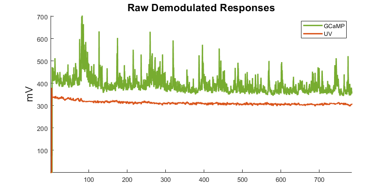
Basic plotting and artifact removal

Make a time array based on number of samples and sample freq of demodulated streams

time = (1:length(data.streams.(GCAMP).data))/data.streams.(GCAMP).fs;

Plot both unprocessed demodulated data streams

figure('Position',[100, 100, 800, 400])
hold on;
p1 = plot(time, data.streams.(GCAMP).data,'color',green,'LineWidth',2);
p2 = plot(time, data.streams.(ISOS).data,'color',red,'LineWidth',2);
title('Raw Demodulated Responses','fontsize',16);
ylabel('mV','fontsize',16);
axis tight;
legend([p1 p2], {'GCaMP','UV'});

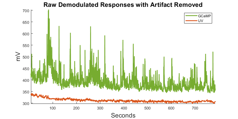
Artifact removal

There is often a large artifact on the onset of LEDs turning on Remove data below a set time t

t = 8; % time threshold below which we will discard
ind = find(time>t,1); % find first index of when time crosses threshold
time = time(ind:end); % reformat vector to only include allowed time
data.streams.(GCAMP).data = data.streams.(GCAMP).data(ind:end);
data.streams.(ISOS).data = data.streams.(ISOS).data(ind:end);

Plot again at new time range

clf;
hold on;
p1 = plot(time, data.streams.(GCAMP).data,'color',green,'LineWidth',2);
p2 = plot(time, data.streams.(ISOS).data,'color',red,'LineWidth',2);
title('Raw Demodulated Responses with Artifact Removed','fontsize',16);
xlabel('Seconds','fontsize',16)
ylabel('mV','fontsize',16);
axis tight;
legend([p1 p2], {'GCaMP','UV'});

Downsample data doing local averaging

Average around every Nth point and downsample Nx

N = 10; % multiplicative for downsampling
data.streams.(GCAMP).data = arrayfun(@(i)...
    mean(data.streams.(GCAMP).data(i:i+N-1)),...
    1:N:length(data.streams.(GCAMP).data)-N+1);
data.streams.(ISOS).data = arrayfun(@(i)...
    mean(data.streams.(ISOS).data(i:i+N-1)),...
    1:N:length(data.streams.(ISOS).data)-N+1);

Decimate time array and match length to demodulated stream

time = time(1:N:end);
time = time(1:length(data.streams.(GCAMP).data));

Detrending and dFF

bls = polyfit(data.streams.(ISOS).data,data.streams.(GCAMP).data,1);
Y_fit_all = bls(1) .* data.streams.(ISOS).data + bls(2);
Y_dF_all = data.streams.(GCAMP).data - Y_fit_all; %dF (units mV) is not dFF

Full dFF according to Lerner et al. 2015 https://dx.doi.org/10.1016/j.cell.2015.07.014 dFF using 405 fit as baseline

dFF = 100*(Y_dF_all)./Y_fit_all;
std_dFF = std(double(dFF));

Turn Licking Events into Lick Bouts

Make a continuous time series of Licking TTL events (epocs) and plot

LICK_on = data.epocs.(LICK).onset;
LICK_off = data.epocs.(LICK).offset;
LICK_x = reshape(kron([LICK_on, LICK_off], [1, 1])', [], 1);
sz = length(LICK_on);
d = data.epocs.(LICK).data';
y_scale = 10; %adjust according to data needs
y_shift = -20; %scale and shift are just for aesthetics
LICK_y = reshape([zeros(1, sz); d; d; zeros(1, sz)], 1, []);

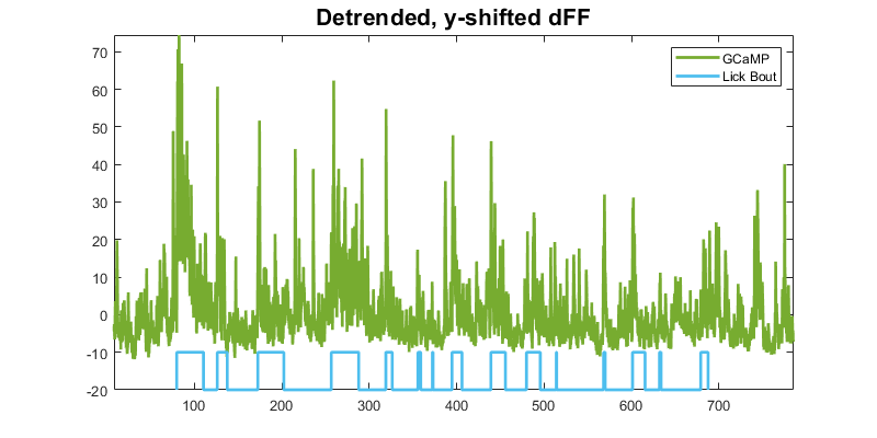
First subplot in a series: dFF with lick epocs

figure('Position',[100, 100, 800, 400]);
p1 = plot(time, dFF, 'Color',green,'LineWidth',2); hold on;
p2 = plot(LICK_x, y_scale*(LICK_y) + y_shift,'color',cyan,'LineWidth',2);
title('Detrended, y-shifted dFF','fontsize',16);
legend([p1 p2],'GCaMP','Lick Epoc');
axis tight

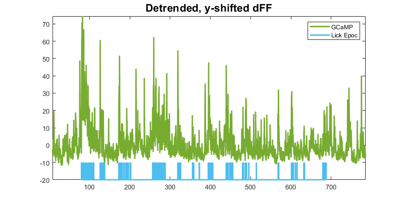
Now combine lick epocs that happen in close succession to make a single on/off event (a lick BOUT). Top view logic: if difference between consecutive lick onsets is below a certain time threshold and there was more than one lick in a row, then consider it as one bout, otherwise it is its own bout. Also, make sure a minimum number of licks was reached to call it a bout.

Make a new epoc event in the data structure

LICK_EVENT = 'Lick_Event';
data.epocs.(LICK_EVENT).name = LICK_EVENT;
data.epocs.(LICK_EVENT).onset = [];
data.epocs.(LICK_EVENT).offset = [];
data.epocs.(LICK_EVENT).typeStr = data.epocs.(LICK).typeStr;
data.epocs.(LICK_EVENT).data = [];

Find differences in onsets and threshold for major difference indices

lick_on_diff = diff(data.epocs.(LICK).onset);
BOUT_TIME_THRESHOLD = 10; % example bout time threshold, in seconds
lick_diff_ind = find(lick_on_diff >= BOUT_TIME_THRESHOLD);

Make an onset/ offset array based on threshold indices

diff_ind_i = 1;
for i = 1:length(lick_diff_ind)
    % BOUT onset is thresholded onset index of lick epoc event
    data.epocs.(LICK_EVENT).onset(i) = data.epocs.(LICK).onset(diff_ind_i);

    % BOUT offset is thresholded offset of lick event before next onset
    data.epocs.(LICK_EVENT).offset(i) = ...
        data.epocs.(LICK).offset(lick_diff_ind(i));

    data.epocs.(LICK_EVENT).data(i) = 1; % set the data value, arbitrary 1
    diff_ind_i = lick_diff_ind(i) + 1; % increment the index
end

% Special case for last event to handle lick event offset indexing
data.epocs.(LICK_EVENT).onset = [data.epocs.(LICK_EVENT).onset, ...
   data.epocs.(LICK).onset(lick_diff_ind(end)+1)];
data.epocs.(LICK_EVENT).offset = [data.epocs.(LICK_EVENT).offset, ...
   data.epocs.(LICK).offset(end)];
data.epocs.(LICK_EVENT).data = [data.epocs.(LICK_EVENT).data, 1];

% Transpose the arrays to make them column vectors like other epocs
data.epocs.(LICK_EVENT).onset = data.epocs.(LICK_EVENT).onset';
data.epocs.(LICK_EVENT).offset = data.epocs.(LICK_EVENT).offset';
data.epocs.(LICK_EVENT).data = data.epocs.(LICK_EVENT).data';

% Note that for speed the previous section could be replaced with these three lines
% data.epocs.(LICK_EVENT).onset = data.epocs.(LICK).onset([1; lick_diff_ind+1]);
% data.epocs.(LICK_EVENT).offset = data.epocs.(LICK).offset([lick_diff_ind; end]);
% data.epocs.(LICK_EVENT).data = ones(1, length(data.epocs.(LICK_EVENT).onset))';

Now determine if it was a 'real' bout or not by thresholding by some user-set number of licks in a row

MIN_LICK_THRESH = 4; % four licks or more make a bout
licks_array = zeros(length(data.epocs.(LICK_EVENT).onset),1);
for i = 1:length(data.epocs.(LICK_EVENT).onset)
    % Find number of licks in licks_array between onset ond offset of
    % Our new lick BOUT (LICK_EVENT)
    licks_array(i) = numel(find(data.epocs.(LICK).onset >=...
        data.epocs.(LICK_EVENT).onset(i) & data.epocs.(LICK).onset <=...
        data.epocs.(LICK_EVENT).offset(i)));
end

Remove onsets, offsets, and data of thrown out events. MATLAB can use booleans for indexing. Cool!

data.epocs.(LICK_EVENT).onset((licks_array < MIN_LICK_THRESH)) = [];
data.epocs.(LICK_EVENT).offset((licks_array < MIN_LICK_THRESH)) = [];
data.epocs.(LICK_EVENT).data((licks_array < MIN_LICK_THRESH)) = [];

Make continuous time series for lick BOUTS for plotting

LICK_EVENT_on = data.epocs.(LICK_EVENT).onset;
LICK_EVENT_off = data.epocs.(LICK_EVENT).offset;
LICK_EVENT_x = reshape(kron([LICK_EVENT_on,LICK_EVENT_off],[1, 1])',[],1);
sz = length(LICK_EVENT_on);
d = data.epocs.(LICK_EVENT).data';
LICK_EVENT_y = reshape([zeros(1, sz); d; d; zeros(1, sz)], 1, []);

Next step: dFF with newly defined lick bouts

clf;
p1 = plot(time, dFF,'Color',green,'LineWidth',2);
hold on;
p2 = plot(LICK_EVENT_x, y_scale*(LICK_EVENT_y) + y_shift,...
    'color',cyan,'LineWidth',2);
title('Detrended, y-shifted dFF','fontsize',16);
legend([p1 p2],'GCaMP', 'Lick Bout');
axis tight

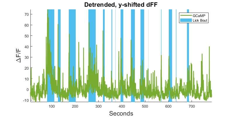
Making nice area fills instead of epocs for aesthetics. Newer versions of MATLAB can use alpha on area fills, which could be desirable

clf;
hold on;
dFF_min = min(dFF);
dFF_max = max(dFF);
for i = 1:numel(data.epocs.(LICK_EVENT).onset)
    h1(i) = area([data.epocs.(LICK_EVENT).onset(i) ...
        data.epocs.(LICK_EVENT).offset(i)], [dFF_max dFF_max], ...
        dFF_min, 'FaceColor',cyan,'edgecolor', 'none');
end
p1 = plot(time, dFF,'Color',green,'LineWidth',2);
title('Detrended, y-shifted dFF','fontsize',16);
legend([p1 h1(1)],'GCaMP', 'Lick Bout');
ylabel('\DeltaF/F','fontsize',16)
xlabel('Seconds','fontsize',16);
axis tight

Time Filter Around Lick Bout Epocs

Note that we are using dFF of the full time-series, not peri-event dFF where f0 is taken from a pre-event baseline period. That is done in another fiber photometry data analysis example.

PRE_TIME = 5; % ten seconds before event onset
POST_TIME = 10; % ten seconds after
fs = data.streams.(GCAMP).fs/N; % recall we downsampled by N = 100 earlier
% time span for peri-event filtering, PRE and POST
TRANGE = [-1*PRE_TIME*floor(fs),POST_TIME*floor(fs)];

Pre-allocate memory

trials = numel(data.epocs.(LICK_EVENT).onset);
dFF_snips = cell(trials,1);
array_ind = zeros(trials,1);
pre_stim = zeros(trials,1);
post_stim = zeros(trials,1);

Make stream snips based on trigger onset

for i = 1:trials
    % If the bout cannot include pre-time seconds before event, make zero
    if data.epocs.(LICK_EVENT).onset(i) < PRE_TIME
        dFF_snips{i} = single(zeros(1,(TRANGE(2)-TRANGE(1))));
        continue
    else
        % Find first time index after bout onset
        array_ind(i) = find(time > data.epocs.(LICK_EVENT).onset(i),1);

        % Find index corresponding to pre and post stim durations
        pre_stim(i) = array_ind(i) + TRANGE(1);
        post_stim(i) = array_ind(i) + TRANGE(2);
        dFF_snips{i} = dFF(pre_stim(i):post_stim(i));
    end
end

Make all snippet cells the same size based on minimum snippet length

minLength = min(cellfun('prodofsize', dFF_snips));
dFF_snips = cellfun(@(x) x(1:minLength), dFF_snips, 'UniformOutput',false);

% Convert to a matrix and get mean
allSignals = cell2mat(dFF_snips);
mean_allSignals = mean(allSignals);
std_allSignals = std(mean_allSignals);

% Make a time vector snippet for peri-events
peri_time = (1:length(mean_allSignals))/fs - PRE_TIME;

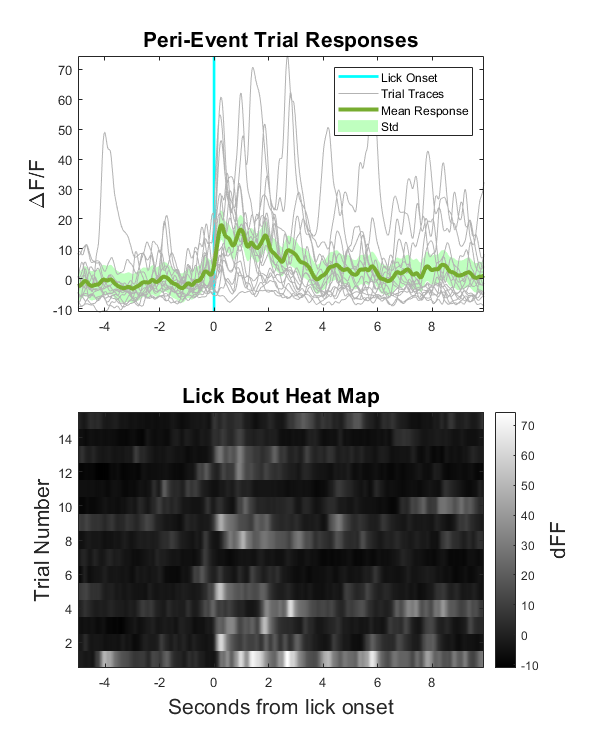
Make a Peri-Event Stimulus Plot and Heat Map

% Make a standard deviation fill for mean signal
figure('Position',[100, 100, 600, 750])
subplot(2,1,1)
xx = [peri_time, fliplr(peri_time)];
yy = [mean_allSignals + std_allSignals,...
    fliplr(mean_allSignals - std_allSignals)];
h = fill(xx, yy, 'g'); % plot this first for overlay purposes
hold on;
set(h, 'facealpha', 0.25, 'edgecolor', 'none');

% Set specs for min and max value of event line.
% Min and max of either std or one of the signal snip traces
linemin = min(min(min(allSignals)),min(yy));
linemax = max(max(max(allSignals)),max(yy));

% Plot the line next
l1 = line([0 0], [linemin, linemax],...
    'color','cyan', 'LineStyle', '-', 'LineWidth', 2);
% Plot the signals and the mean signal
p1 = plot(peri_time, allSignals', 'color', gray1);
p2 = plot(peri_time, mean_allSignals, 'color', green, 'LineWidth', 3);
hold off;

% Make a legend and do other plot things
legend([l1, p1(1), p2, h],...
    {'Lick Onset','Trial Traces','Mean Response','Std'},...
    'Location','northeast');
title('Peri-Event Trial Responses','fontsize',16);
ylabel('\DeltaF/F','fontsize',16);
axis tight;
% Make an invisible colorbar so this plot aligns with one below it
temp_cb = colorbar('Visible', 'off');

% Heat map
subplot(2,1,2)
imagesc(peri_time, 1, allSignals); % this is the heatmap
set(gca,'YDir','normal') % put the trial numbers in better order on y-axis
colormap(gray()) % colormap otherwise defaults to perula
title('Lick Bout Heat Map','fontsize',16)
ylabel('Trial Number','fontsize',16)
xlabel('Seconds from lick onset','fontsize',16)
cb = colorbar;
ylabel(cb, 'dFF','fontsize',16)
axis tight;