Fiber Photometry Epoch Averaging Example

This example goes through fiber photometry analysis using techniques such as data smoothing, bleach detrending, and z-score analysis.
The epoch averaging was done using TDTfilter.

Author Contributions:
TDT, David Root, and the Morales Lab contributed to the writing and/or conceptualization of the code.
The signal processing pipeline was inspired by the workflow developed by David Barker et al. (2017) for the Morales Lab.
The data used in the example were provided by David Root.

Author Information:
David H. Root
Assistant Professor
Department of Psychology & Neuroscience
University of Colorado, Boulder
Lab Website: https://www.root-lab.org
david.root@colorado.edu

About the authors:
The Root lab and Morales lab investigate the neurobiology of reward, aversion, addiction, and depression.

TDT edits all user submissions in coordination with the contributing author(s) prior to publishing.

Download M File

Housekeeping

Clear workspace and close existing figures. Add SDK directories to MATLAB path.

close all; clear all; clc;
[MAINEXAMPLEPATH,name,ext] = fileparts(cd); % \TDTMatlabSDK\Examples
DATAPATH = fullfile(MAINEXAMPLEPATH, 'ExampleData'); % \TDTMatlabSDK\Examples\ExampleData
[SDKPATH,name,ext] = fileparts(MAINEXAMPLEPATH); % \TDTMatlabSDK
addpath(genpath(SDKPATH));

Importing the Data

This example assumes you downloaded our example data sets and extracted it into the \TDTMatlabSDK\Examples directory. To import your own data, replace 'BLOCKPATH' with the path to your own data block.

In Synapse, you can find the block path in the database. Go to Menu → History. Find your block, then Right-Click → Copy path to clipboard.

BLOCKPATH = fullfile(DATAPATH,'FiPho-180416');

Setup the variables for the data you want to extract

We will extract two different stream stores surrounding the 'PtAB' epoch event. We are interested in a specific event code for the shock onset.

REF_EPOC = 'PtAB'; % event store name. This holds behavioral codes that are
% read through Ports A & B on the front of the RZ
SHOCK_CODE = 64959; % shock onset event code we are interested in
STREAM_STORE1 = 'x4054'; % name of the 405 store
STREAM_STORE2 = 'x4654'; % name of the 465 store
TRANGE = [-10 20]; % window size [start time relative to epoc onset, window duration]
BASELINE_PER = [-10 -6]; % baseline period within our window
ARTIFACT = Inf; % optionally set an artifact rejection level

% Now read the specified data from our block into a MATLAB structure.
data = TDTbin2mat(BLOCKPATH, 'TYPE', {'epocs', 'scalars', 'streams'});

read from t=0.00s to t=583.86s

Use TDTfilter to extract data around our epoc event

Using the 'TIME' parameter extracts data only from the time range around our epoc event. Use the 'VALUES' parameter to specify allowed values of the REF_EPOC to extract. For stream events, the chunks of data are stored in cell arrays structured as data.streams.(STREAM_STORE1).filtered

data = TDTfilter(data, REF_EPOC, 'VALUES', SHOCK_CODE, 'TIME', TRANGE);

Optionally remove artifacts. If any waveform is above ARTIFACT level, or below -ARTIFACT level, remove it from the data set.

art1 = ~cellfun('isempty', cellfun(@(x) x(x>ARTIFACT), data.streams.(STREAM_STORE1).filtered, 'UniformOutput',false));
art2 = ~cellfun('isempty', cellfun(@(x) x(x<-ARTIFACT), data.streams.(STREAM_STORE1).filtered, 'UniformOutput',false));
good = ~art1 & ~art2;
data.streams.(STREAM_STORE1).filtered = data.streams.(STREAM_STORE1).filtered(good);

art1 = ~cellfun('isempty', cellfun(@(x) x(x>ARTIFACT), data.streams.(STREAM_STORE2).filtered, 'UniformOutput',false));
art2 = ~cellfun('isempty', cellfun(@(x) x(x<-ARTIFACT), data.streams.(STREAM_STORE2).filtered, 'UniformOutput',false));
good2 = ~art1 & ~art2;
data.streams.(STREAM_STORE2).filtered = data.streams.(STREAM_STORE2).filtered(good2);

numArtifacts = sum(~good) + sum(~good2);

Applying a time filter to a uniformly sampled signal means that the length of each segment could vary by one sample. Let's find the minimum length so we can trim the excess off before calculating the mean.

minLength1 = min(cellfun('prodofsize', data.streams.(STREAM_STORE1).filtered));
minLength2 = min(cellfun('prodofsize', data.streams.(STREAM_STORE2).filtered));
data.streams.(STREAM_STORE1).filtered = cellfun(@(x) x(1:minLength1), data.streams.(STREAM_STORE1).filtered, 'UniformOutput',false);
data.streams.(STREAM_STORE2).filtered = cellfun(@(x) x(1:minLength2), data.streams.(STREAM_STORE2).filtered, 'UniformOutput',false);

allSignals = cell2mat(data.streams.(STREAM_STORE1).filtered');

% downsample 10x and average 405 signal
N = 10;
F405 = zeros(size(allSignals(:,1:N:end-N+1)));
for ii = 1:size(allSignals,1)
    F405(ii,:) = arrayfun(@(i) mean(allSignals(ii,i:i+N-1)),1:N:length(allSignals)-N+1);
end
minLength1 = size(F405,2);

% Create mean signal, standard error of signal, and DC offset of 405 signal
meanSignal1 = mean(F405);
stdSignal1 = std(double(F405))/sqrt(size(F405,1));
dcSignal1 = mean(meanSignal1);

% downsample 10x and average 465 signal
allSignals = cell2mat(data.streams.(STREAM_STORE2).filtered');
F465 = zeros(size(allSignals(:,1:N:end-N+1)));
for ii = 1:size(allSignals,1)
    F465(ii,:) = arrayfun(@(i) mean(allSignals(ii,i:i+N-1)),1:N:length(allSignals)-N+1);
end
minLength2 = size(F465,2);

% Create mean signal, standard error of signal, and DC offset of 465 signal
meanSignal2 = mean(F465);
stdSignal2 = std(double(F465))/sqrt(size(F465,1));
dcSignal2 = mean(meanSignal2);

Plot Epoch Averaged Response

% Create the time vector for each stream store
ts1 = TRANGE(1) + (1:minLength1) / data.streams.(STREAM_STORE1).fs*N;
ts2 = TRANGE(1) + (1:minLength2) / data.streams.(STREAM_STORE2).fs*N;

% Subtract DC offset to get signals on top of one another
meanSignal1 = meanSignal1 - dcSignal1;
meanSignal2 = meanSignal2 - dcSignal2;

% Plot the 405 and 465 average signals
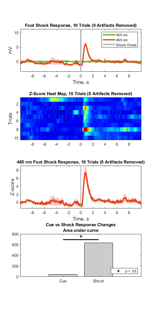
figure;
subplot(4,1,1)
plot(ts1, meanSignal1, 'color',[0.4660, 0.6740, 0.1880], 'LineWidth', 3); hold on;
plot(ts2, meanSignal2, 'color',[0.8500, 0.3250, 0.0980], 'LineWidth', 3);

% Plot vertical line at epoch onset, time = 0
line([0 0], [min(F465(:) - dcSignal2), max(F465(:)) - dcSignal2], 'Color', [.7 .7 .7], 'LineStyle','-', 'LineWidth', 3)

% Make a legend
legend('405 nm','465 nm','Shock Onset', 'AutoUpdate', 'off');

% Create the standard error bands for the 405 signal
XX = [ts1, fliplr(ts1)];
YY = [meanSignal1 + stdSignal1, fliplr(meanSignal1 - stdSignal1)];

% Plot filled standard error bands.
h = fill(XX, YY, 'g');
set(h, 'facealpha',.25,'edgecolor','none')

% Repeat for 465
XX = [ts2, fliplr(ts2)];
YY = [meanSignal2 + stdSignal2, fliplr(meanSignal2 - stdSignal2)];
h = fill(XX, YY, 'r');
set(h, 'facealpha',.25,'edgecolor','none')

% Finish up the plot
axis tight
xlabel('Time, s','FontSize',12)
ylabel('mV', 'FontSize', 12)
title(sprintf('Foot Shock Response, %d Trials (%d Artifacts Removed)', numel(data.streams.(STREAM_STORE1).filtered), numArtifacts))
set(gcf, 'Position',[100, 100, 800, 500])

% Heat Map based on z score of 405 fit subtracted 465

% Fitting 405 channel onto 465 channel to detrend signal bleaching
% Scale and fit data
% Algorithm sourced from Tom Davidson's Github:
% https://github.com/tjd2002/tjd-shared-code/blob/master/matlab/photometry/FP_normalize.m

bls = polyfit(F405(1:end), F465(1:end), 1);
Y_fit_all = bls(1) .* F405 + bls(2);
Y_dF_all = F465 - Y_fit_all;

zall = zeros(size(Y_dF_all));
for i = 1:size(Y_dF_all,1)
    ind = ts2(1,:) < BASELINE_PER(2) & ts2(1,:) > BASELINE_PER(1);
    zb = mean(Y_dF_all(i,ind)); % baseline period mean (-10sec to -6sec)
    zsd = std(Y_dF_all(i,ind)); % baseline period stdev
    zall(i,:)=(Y_dF_all(i,:) - zb)/zsd; % Z score per bin
end

% Standard error of the z-score
zerror = std(zall)/sqrt(size(zall,1));

% Plot heat map
subplot(4,1,2)

imagesc(ts2, 1, zall);
colormap('jet'); % c1 = colorbar;
title(sprintf('Z-Score Heat Map, %d Trials (%d Artifacts Removed)', numel(data.streams.(STREAM_STORE1).filtered), numArtifacts));
ylabel('Trials', 'FontSize', 12);

% Fill band values for second subplot. Doing here to scale onset bar
% correctly
XX = [ts2, fliplr(ts2)];
YY = [mean(zall)-zerror, fliplr(mean(zall)+zerror)];

subplot(4,1,3)
plot(ts2, mean(zall), 'color',[0.8500, 0.3250, 0.0980], 'LineWidth', 3); hold on;
line([0 0], [min(YY), max(YY)], 'Color', [.7 .7 .7], 'LineWidth', 2)

h = fill(XX, YY, 'r');
set(h, 'facealpha',.25,'edgecolor','none')

% Finish up the plot
axis tight
xlabel('Time, s','FontSize',12)
ylabel('Z-score', 'FontSize', 12)
title(sprintf('465 nm Foot Shock Response, %d Trials (%d Artifacts Removed)', numel(data.streams.(STREAM_STORE1).filtered), numArtifacts))
%c2 = colorbar;

% Quantify changes as area under the curve for cue (-5 sec) and shock (0 sec)
AUC=[]; % cue, shock
AUC(1,1)=trapz(mean(zall(:,ts2(1,:) < -3 & ts2(1,:) > -5)));
AUC(1,2)=trapz(mean(zall(:,ts2(1,:) > 0 & ts2(1,:) < 2)));
subplot(4,1,4);
hBar = bar(AUC, 'FaceColor', [.8 .8 .8]);

% Run a two-sample T-Test
[h,p,ci,stats] = ttest2(mean(zall(:,ts2(1,:) < -3 & ts2(1,:) > -5)),mean(zall(:,ts2(1,:) > 0 & ts2(1,:) < 2)));

% Plot significance bar if p < .05
hold on;
centers = get(hBar, 'XData');
plot(centers(1:2), [1 1]*AUC(1,2)*1.1, '-k', 'LineWidth', 2)
p1 = plot(mean(centers(1:2)), AUC(1,2)*1.2, '*k');
set(gca,'xticklabel',{'Cue','Shock'});
title({'Cue vs Shock Response Changes', 'Area under curve'})
legend(p1, 'p < .05','Location','southeast');

set(gcf, 'Position',[100, 100, 500, 1000])