Snippet Plot Example
Import snippet data into MATLAB using TDTbin2mat
Sort snippets based on channel number and sort code for any number of channels and sort codes
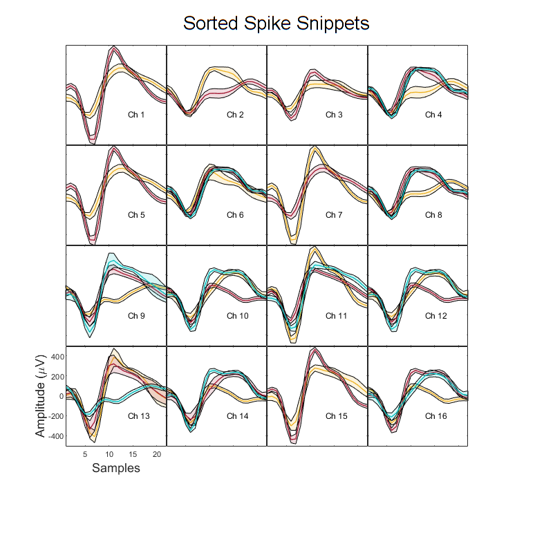
Plot the average waveform shape and standard deviation for 16 channels and three sort codes
Good for spike sorting and first-pass visualization of sorted waveforms
Housekeeping
Clear workspace and close existing figures. Add SDK directories to MATLAB path.
close all; clear all; clc;
[MAINEXAMPLEPATH,name,ext] = fileparts(cd); % \TDTMatlabSDK\Examples
DATAPATH = fullfile(MAINEXAMPLEPATH, 'ExampleData'); % \TDTMatlabSDK\Examples\ExampleData
[SDKPATH,name,ext] = fileparts(MAINEXAMPLEPATH); % \TDTMatlabSDK
addpath(genpath(SDKPATH));
Importing the Data
This example assumes you downloaded our example data sets and extracted it into the \TDTMatlabSDK\Examples directory. To import your own data, replace 'BLOCKPATH' with the path to your own data block.
In Synapse, you can find the block path in the database. Go to Menu → History. Find your block, then Right-Click → Copy path to clipboard.
BLOCKPATH = fullfile(DATAPATH,'Algernon-180308-130351');
Now read snippet data into a MATLAB structure called 'data'.
data = TDTbin2mat(BLOCKPATH, 'TYPE', {'snips'});
read from t=0.00s to t=61.23s
And that's it! Your data is now in MATLAB. The rest of the code describes sorting snippets based on channel number and sort code, then plotting a subselection of three sort codes.
Spike Snippet Sorting
Collect waveforms, averages, standard deviation, and snippet times of all snippets, sorted by channel and sortcode number.
% Note: If you want a pile plot of *ALL* snippets (every channel), use this:
% figure;
% plot(samples, data.snips.eNe1.data(:,:));

% Pull field name as string from snip store
SNIP_STORE = fieldnames(data.snips);
SNIP_STORE = SNIP_STORE{1};

% Useful variables
numchans = single(max(data.snips.(SNIP_STORE).chan));
if numchans > 64
    warning('This display function is only good for 64 channels or fewer. Truncating to 64 channels');
    numchans = 64;
end

nsamples = length(data.snips.(SNIP_STORE).data(1,:));
sorts = sort(unique(data.snips.(SNIP_STORE).sortcode))';

% Remove unsorted and outliers from analysis unless it's the only one
if numel(sorts) ~= 1
    sorts(sorts==0 | sorts==31) = [];
end

% Declare stores for sort codes, averages, standard deviations, and timestamps
sorted_stores = cell(numchans, numel(sorts));
store_averages = cell(numchans, numel(sorts));
sorted_stdp = cell(numchans, numel(sorts));
sorted_stdn = cell(numchans, numel(sorts));
snip_times = cell(numchans, numel(sorts));
snip_isi = cell(numchans, numel(sorts));

% Filter based on channel and sort code
for chan = 1:numchans
    for sort_ind = 1:numel(sorts)
        sort_code = sorts(sort_ind);
        % Create index for data that matches current channel and sortcode
        i = find(data.snips.(SNIP_STORE).chan == chan & data.snips.(SNIP_STORE).sortcode == sort_code);
        sorted_stores{chan, sort_code} = 1e6*data.snips.(SNIP_STORE).data(i,:); % scaled to uV
        store_averages{chan, sort_code} = sum(sorted_stores{chan, sort_code}/length(sorted_stores{chan, sort_code}));
        if size(sorted_stores{chan, sort_code}, 1) > 1
            sorted_stdp{chan, sort_code} = std(sorted_stores{chan, sort_code}) + store_averages{chan, sort_code};
            sorted_stdn{chan, sort_code} = store_averages{chan, sort_code} - std(sorted_stores{chan, sort_code});
        else
            sorted_stdp{chan, sort_code} = zeros(1, size(sorted_stores{chan, sort_code},2));
            sorted_stdn{chan, sort_code} = zeros(1, size(sorted_stores{chan, sort_code},2));
        end
        % Find timestamps of snips
        snip_times{chan, sort_code} = data.snips.(SNIP_STORE).ts(i);

        % Inter-spike Interval of sorted snips
        snip_isi{chan,sort_code} = diff(snip_times{chan,sort_code});
    end
end

% Use this code block to extract unsorted and outlier snips
% unsorted = cell(numchans,1);
% outliers = cell(numchans,1);
%
% for CHANNEL = 1:numchans
%     i = data.snips.(SNIP_STORE).chan == CHANNEL & data.snips.(SNIP_STORE).sortcode == 0;
%     unsorted{CHANNEL, 1} = data.snips.(SNIP_STORE).data(i,:);
%
%     j = data.snips.(SNIP_STORE).chan == CHANNEL & data.snips.(SNIP_STORE).sortcode == 31;
%     outliers{CHANNEL, 1} = data.snips.(SNIP_STORE).data(j,:);
% end
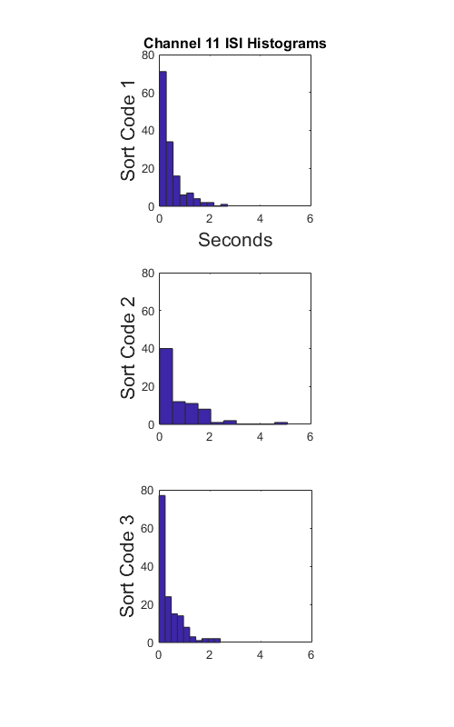
Generate an ISI histogram for selected channels
Look at ISI histogram for first 3 sort codes
PLOT_CHANS = [11]; % change to 1:numchans to plot all of them

ax = cell(1,3);
for chan = PLOT_CHANS
    figure('Name','ISI Histograms','Position',[900, 100, 500, 800]);
    for sort_ind = 1:size(snip_isi,2)
        % skip sort code if there are none
        if size(snip_isi{chan, sort_ind},1) == 0, continue, end

        % make histogram on new subplot
        ax{sort_ind} = subplot(3,1,sort_ind);
        hist(snip_isi{chan,sort_ind});

        if sort_ind == 1
            title(sprintf('Channel %d ISI Histograms',chan),'FontSize',12)
            xlabel('Seconds','FontSize',16)
        end
        ylabel(sprintf('Sort Code %d',sorts(sort_ind)),'FontSize',16)
        axis square
    end
    linkaxes([ax{:}],'xy');
end
Waveform Plots
Create filled waveform plots with channels and sortcodes
Waveforms will be the average waveform of all snippets for each sortcode for each channel, with a standard deviation fill around it
Note: The plot below uses up to 64 channels and 3 sort codes but can be modified
% Samples array for x-axis of fill plots
sample_arr = 1:nsamples;
XX = [sample_arr, fliplr(sample_arr)];

% set plot locations based on channel count
numcols = double(ceil(sqrt(numchans)));
numrows = double(ceil(numchans/numcols));
spc = sqrt(numrows*numcols)+1.5;
indt1 = 1/(numrows*numrows);
indt2 = 0.8-indt1;

h = figure('Name','Sorted Spike Snippets','Position', [100, 100, 800, 800]);

% Add master title to subplots using figure uicontrol
uicontrol('Style','text','String','Sorted Spike Snippets',...
    'FontSize',20','HorizontalAlignment','center','Units','normalized',...
    'Position', [0 .93 1 .05],'BackgroundColor',[1 1 1]);

% Default colors for sort codes 1, 2, 3
colors = {[0.9290, 0.6940, 0.1250],[0.6350, 0.0780, 0.1840],[0, 0.75, 0.75]};

max_axis = zeros(1,4);
ax = zeros(1, numchans);

row = 1;
col = 1;
last_sort = min(size(snip_isi,2),3);
for chan = 1:numchans
    for sort_ind = 1:last_sort
        % Used for filling Std Dev in with Fill later
        YY = [sorted_stdp{chan,sort_ind}, fliplr(sorted_stdn{chan,sort_ind})];

        pos = [col/spc-indt1 indt2-(row-1)/spc 1/spc 1/spc];
        ax(chan) = subplot('Position',pos);

        % create an empty axis if no sort codes found
        if all(cell2mat(store_averages(chan,1:last_sort)) == 0) && sort_ind == last_sort
            plot(zeros(size(store_averages{chan,sort_ind})),'w','LineWidth',1);
        else
            if ~all(store_averages{chan,sort_ind} == 0)
                % Std dev fill around averaged waveform
                h = fill(XX, YY, colors{sort_ind});
                set(h, 'facealpha', .15); %set transparency of fill plot
                hold on;
                plot(store_averages{chan,sort_ind},'color',colors{sort_ind},'LineWidth',1);
            end
        end
        if sort_ind == last_sort
            % Channel labels
            text(15-sqrt(col), -200, sprintf('Ch %d',chan), 'FontSize', 14/((numrows^(1/3))));
            axis square;
            axis tight;
        end

        % Only add axis labels on left column and bottom row
        if row == numrows && col == 1
            xlabel('Samples','FontSize',16/((numrows^(1/8))));
            ylabel('Amplitude (\muV)','FontSize',16/((numrows^(1/8))));
        else
            % Get rid of the numbers but leave the ticks.
            set(ax(chan),'Xticklabel',[]);
            set(ax(chan),'Yticklabel',[]);
        end
    end

    % fill one row at a time, go to the next row when col == numcols
    if col == numcols
        row = row+1;
        col = 1;
    else
        col = col+1;
    end

end
% use same axes for all plots
linkaxes(ax, 'xy');