Averaging Example

Import stream and epoc data into MATLAB using TDTbin2mat
Plot the average waveform around the epoc event
Good for Evoked Potential detection

Download M File

Housekeeping

Clear workspace and close existing figures. Add SDK directories to MATLAB path.

close all; clear all; clc;
[MAINEXAMPLEPATH,name,ext] = fileparts(cd); % \TDTMatlabSDK\Examples
DATAPATH = fullfile(MAINEXAMPLEPATH, 'ExampleData'); % \TDTMatlabSDK\Examples\ExampleData
[SDKPATH,name,ext] = fileparts(MAINEXAMPLEPATH); % \TDTMatlabSDK
addpath(genpath(SDKPATH));

Importing the Data

This example assumes you downloaded our example data sets and extracted it into the \TDTMatlabSDK\Examples directory. To import your own data, replace 'BLOCKPATH' with the path to your own data block.

In Synapse, you can find the block path in the database. Go to Menu → History. Find your block, then Right-Click → Copy path to clipboard.

BLOCKPATH = fullfile(DATAPATH,'Algernon-180308-130351');

Set up the variables for the data you want to extract. We will extract channel 3 from the LFP1 stream data store, created by the Neural Stream Processor gizmo, and use our PulseGen epoc event ('PC0/') as our stimulus onset.

REF_EPOC = 'PC0/';
STREAM_STORE = 'LFP1';
CHANNEL = 3;
ARTIFACT = Inf; % optionally set an artifact rejection level
TRANGE = [-0.3, 0.8]; % window size [start time relative to epoc onset, window duration]

Now read the specified data from our block into a MATLAB structure.

data = TDTbin2mat(BLOCKPATH, 'TYPE', {'epocs', 'scalars', 'streams'}, 'CHANNEL', CHANNEL);

read from t=0.00s to t=61.23s

Use TDTfilter to extract data around our epoc event

Using the 'TIME' parameter extracts data only from the time range around our epoc event. For stream events, the chunks of data are stored in cell arrays.

data = TDTfilter(data, REF_EPOC, 'TIME', TRANGE);

Optionally remove artifacts.

art1 = ~cellfun('isempty', cellfun(@(x) x(x>ARTIFACT), data.streams.(STREAM_STORE).filtered, 'UniformOutput',false));
art2 = ~cellfun('isempty', cellfun(@(x) x(x<-ARTIFACT), data.streams.(STREAM_STORE).filtered, 'UniformOutput',false));
good = ~art1 & ~art2;
data.streams.(STREAM_STORE).filtered = data.streams.(STREAM_STORE).filtered(good);
numArtifacts = sum(~good);

Applying a time filter to a uniformly sampled signal means that the length of each segment could vary by one sample. Let's find the minimum length so we can trim the excess off before calculating the mean.

minLength = min(cellfun('prodofsize', data.streams.(STREAM_STORE).filtered));
data.streams.(STREAM_STORE).filtered = cellfun(@(x) x(1:minLength), data.streams.(STREAM_STORE).filtered, 'UniformOutput',false);

Find the average signal.

allSignals = cell2mat(data.streams.(STREAM_STORE).filtered');
meanSignal = mean(allSignals);
stdSignal = std(double(allSignals));

Ready to plot

Create the time vector.

ts = TRANGE(1) + (1:minLength) / data.streams.(STREAM_STORE).fs;

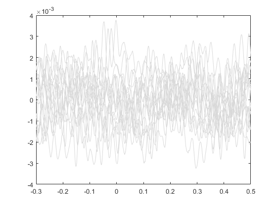
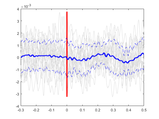
Plot all the signals as gray.

plot(ts, allSignals','Color', [.85 .85 .85]); hold on;

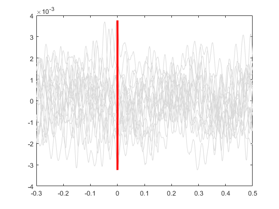
Plot vertical line at time=0.

line([0 0], [min(allSignals(:)), max(allSignals(:))], 'Color', 'r', 'LineStyle','-', 'LineWidth', 3)

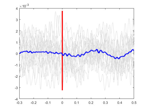
Plot the average signal.

plot(ts, meanSignal, 'b', 'LineWidth', 3)

Plot the standard deviation bands.

plot(ts, meanSignal+stdSignal, 'b--', ts, meanSignal-stdSignal, 'b--');

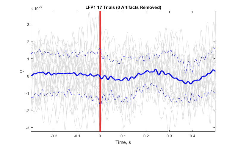
Finish up the plot

axis tight
xlabel('Time, s','FontSize',12)
ylabel('V', 'FontSize', 12)
title(sprintf('%s %d Trials (%d Artifacts Removed)', STREAM_STORE, numel(data.streams.(STREAM_STORE).filtered), numArtifacts))
set(gcf, 'Position',[100, 100, 800, 500])