Filter and Threshold Raw Data Into Snippets

Import raw streaming data into MATLAB using TDTbin2mat
Digitally filter the single unit data using TDTdigitalfilter
Threshold and extract snippets using TDTthresh

Download M File

Housekeeping

Clear workspace and close existing figures. Add SDK directories to MATLAB path.

close all; clear all; clc;
[MAINEXAMPLEPATH,name,ext] = fileparts(cd); % \TDTMatlabSDK\Examples
DATAPATH = fullfile(MAINEXAMPLEPATH, 'ExampleData'); % \TDTMatlabSDK\Examples\ExampleData
[SDKPATH,name,ext] = fileparts(MAINEXAMPLEPATH); % \TDTMatlabSDK
addpath(genpath(SDKPATH));

Importing the Data

This example assumes you downloaded our example data sets and extracted it into the \TDTMatlabSDK\Examples directory. To import your own data, replace 'BLOCKPATH' with the path to your own data block.

In Synapse, you can find the block path in the database. Go to Menu → History. Find your block, then Right-Click → Copy path to clipboard.

BLOCKPATH = fullfile(DATAPATH,'Algernon-180308-130351');

Set up the variables for the data you want to extract. We will extract channel 1 from the Wav1 data store, created by the Stream Data Storage gizmo, and apply our threshold at -125 uV to create 30 sample snippets.

STORE = 'Wav1';
CHANNEL = 1;
THRESH = -125e-6; % define snippet when it crosses this threshold
NPTS = 30; % size of the snippet
OVERLAP = 0; % set to 1 to allow double crossings within same window to count as a different snippet

Now read the specified data from our block into a MATLAB structure.

data = TDTbin2mat(BLOCKPATH, 'STORE', STORE, 'CHANNEL', CHANNEL);

read from t=0.00s to t=61.23s

Use TDTdigitalfilter to filter the streaming waveforms

We are interested in single unit activity in the 300-5000 Hz band.

su = TDTdigitalfilter(data, STORE, [300 5000]);

Use TDTthresh to extract snippet events

Mode is set to 'manual' in this example for extracting snippets around a hard threshold.

su = TDTthresh(su, STORE, 'MODE', 'manual', 'THRESH', THRESH, 'NPTS', NPTS, 'OVERLAP', OVERLAP);

% You could also use 'auto' detection, which sets a moving threshold base
% on a multiple of the RMS of a previous time period. For example,
% set the threshold at 6*RMS of the previous 5 seconds of data
%su = TDTthresh(su, STORE, 'MODE', 'auto', 'POLARITY', -1, 'STD', 6, 'TAU', 5);

window size is 30, without overlap.
using absolute threshold method, set to -125.00 uV.

And that's it! Your data is now in MATLAB and thresholded. TDTthresh adds a new store into the data structure called data.snips.Snip that we will now use for plotting. First, we'll get some properties of the snippets that we'll use later for scatter plots

maxvals = max(su.snips.Snip.data, [], 2)*1e6;
minvals = min(su.snips.Snip.data, [], 2)*1e6;

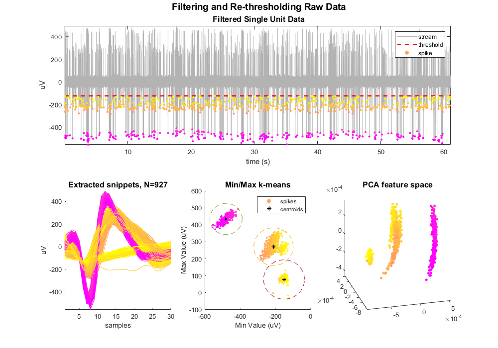
Begin plotting

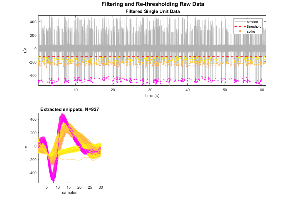
Plot the single unit data with snippet overlay.

subplot(2,3,[1 2 3])
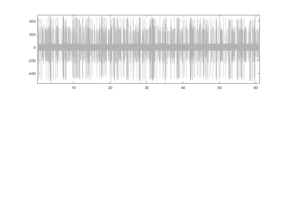
ts = (1:numel(su.streams.(STORE).data(1,:)))/su.streams.(STORE).fs;
plot(ts, su.streams.(STORE).data(1,:)*1e6, 'color', [.7 .7 .7]);
axis([ts(1) ts(end) min(minvals) max(maxvals)]); ax1 = axis();
hold on;

% Position the figure
set(gcf, 'Position', [100 100 1000 700])

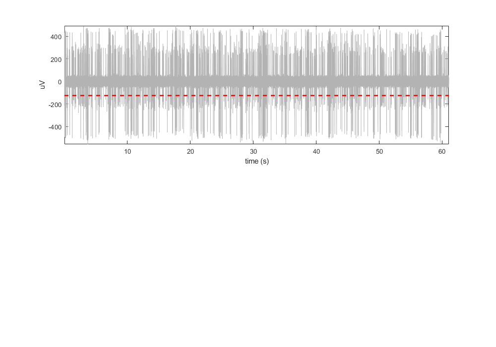
Plot the threshold line.

if numel(su.snips.Snip.thresh) == 1
    thresh = su.snips.Snip.thresh*ones(size(ts));
else
    thresh = su.snips.Snip.thresh;
end
plot(ts, thresh*1e6, 'r--', 'LineWidth', 2)
ylabel('uV');
xlabel('time (s)');

Define a color map based on the minimum values. The dots are not colored by any complex sorting algorithm, just by magnitude. We'll use this coloring to track the snippets through the rest of the plots. This uses the vals2colormap function, which can be found at: <https://github.com/vistalab/vistateach/blob/master/cogneuro/tutorial1_timeseries/vals2colormap.m>.

colors = vals2colormap(minvals, 'spring', [min(minvals)*.9 max(minvals)]);

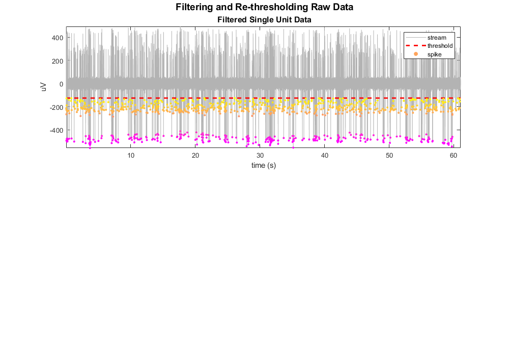
Overlay the min values as dots on the streaming plot.

scatter(su.snips.Snip.ts, minvals, 10, colors, 'filled');

legend({'stream', 'threshold', 'spike'});
% add a fancy latex title
title(['\fontsize{14} Filtering and Re-thresholding Raw Data' char(10) ...
    '\fontsize{12} Filtered Single Unit Data'],'interpreter','tex');

% Alternatively, overlay entire snippets on time window.
%npts = size(su.snips.Snip.data,2);
%for ii = 1:size(su.snips.Snip.data, 1)
%    plot(su.snips.Snip.ts(ii)+((1:npts)-floor(npts/4))/su.snips.Snip.fs, su.snips.Snip.data(ii,:)*1e6, 'color', colors(ii,:));
%end

Plot the extracted snippets.

subplot(2,3,4)
hold on;
for ii = 1:size(su.snips.Snip.data, 1)
    plot(su.snips.Snip.data(ii,:)*1e6, 'color', colors(ii,:));
end
axis tight;
xlabel('samples')
ylabel('uV')
title(sprintf('Extracted snippets, N=%d', ii), 'FontSize', 12)

Do Min/Max k-Means and PCA analysis

Plot snippets in a simple feature space.

subplot(2,3,5)
scatter(minvals, maxvals, 8, colors, 'filled')
xlabel('Min Value (uV)')
ylabel('Max Value (uV)')
title('Min/Max k-means', 'FontSize', 12)
hold on;

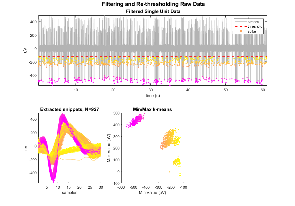
Do k-means for 3 clusters.

rand('seed', 1); % for reproducibility
[idx, C] = kmeans([minvals, maxvals], 3);

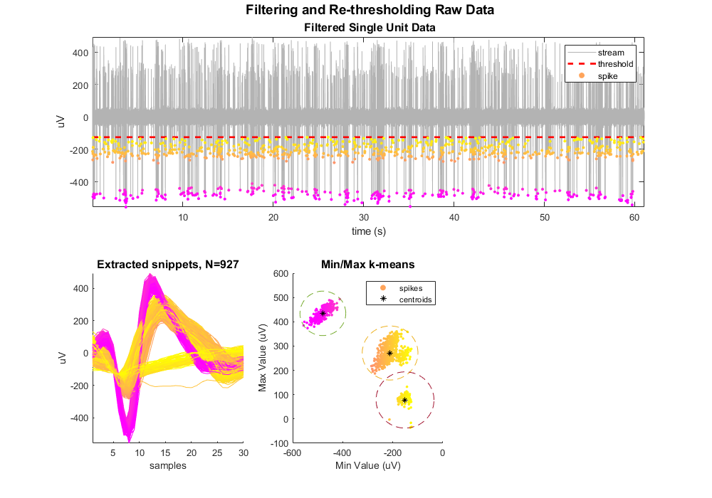
Plot centroids and cluster circles

for ii = 1:max(idx)

    % plot centroid
    scatter(C(ii,1), C(ii,2), 30, '*k');

    % find spike with max distance from center to use as radius for circle
    x_center = C(ii, 1);
    y_center = C(ii, 2);
    curr_mins = minvals(idx==ii);
    curr_maxs = maxvals(idx==ii);
    dist = sqrt((curr_mins - x_center).^2 + (curr_maxs - y_center).^2);
    r = max(dist);

    % plot circle
    th = 0:pi/50:2*pi;
    xunit = r * cos(th) + x_center;
    yunit = r * sin(th) + y_center;
    plot(xunit, yunit, '--');
end
legend({'spikes','centroids'})

Plot snippets in PCA space.

subplot(2,3,6)
hold on;
try
    [coeff,score,latent] = pca(su.snips.Snip.data);  % newer MATLAB uses this
catch
    [coeff,score,latent] = princomp(su.snips.Snip.data);
end

[idx3, C3] = kmeans(score(:,1:3), 3);
for ii = 1:max(idx3)

    % apply sort codes to our data
    su.snips.Snip.sortcode(idx3==ii) = ii;

    % get principle components and color for this cluster
    pca1 = score(idx3==ii,1);
    pca2 = score(idx3==ii,2);
    pca3 = score(idx3==ii,3);
    color = colors(idx3==ii,:);

    % plot dots
    scatter3(pca1, pca2, pca3, 15, color, 'filled')

    % plot centroid
    %scatter3(C3(ii,1), C3(ii,2), C3(ii,3), 75, 'k', 'filled');
end
axis tight;
view([-15 25]); % set initial view on 3-D plot
title('PCA feature space', 'FontSize', 12)

% keep sort code 1 only
idx = su.snips.Snip.sortcode == 1;
su.snips.Snip.sortcode(~idx) = [];
su.snips.Snip.ts(~idx) = [];