Run-Time

The Run-Time layout

The Default Layout

Below is the default Run-Time setup for a fiber photometry gizmo configured to save demodulated streams from LUX LED drivers (405 nm and 465 nm wavelengths) x one PS1 sensor, the broadband raw signal, and the driver parameters (these are not displayed by default). Continuous data streams are displayed in the Flow Plot tab. Order of data streams, or creation of multiple Flow Plots, can be achieved by adjusting RT Layout or FP Setup at Run-Time or Design-Time, respectively.

Note

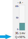
On first run and after turning your LEDs on, you should autoscale the data stream by clicking the icon highlighted by the blue arrow.

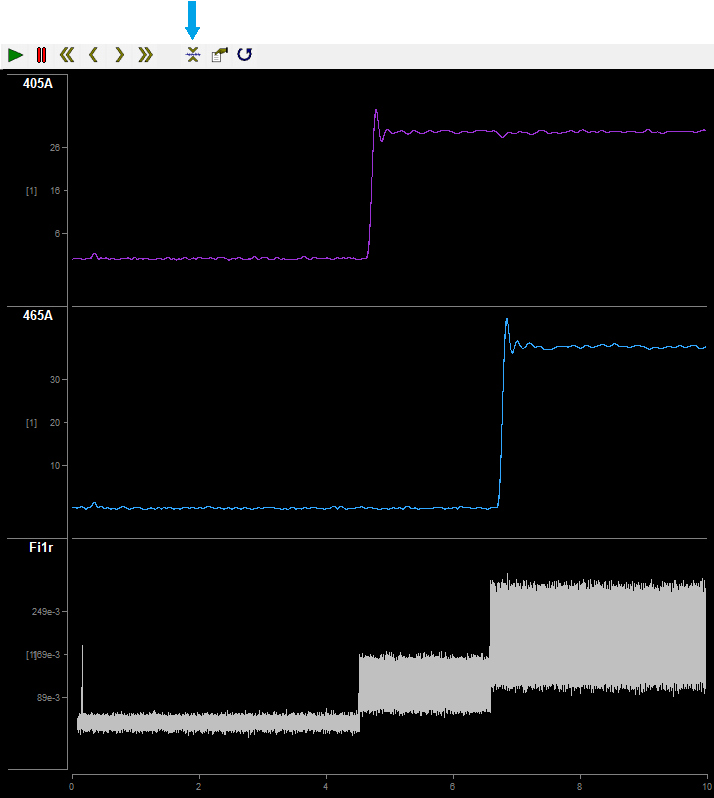
From top to bottom: 405A is the 405 nm driver data demodulated from sensor A; 465A is that for the 465 nm driver; Fi1r is the broadband raw photosensor signals. LED drivers were turned on at ~4.5 seconds and 7 seconds into Preview.

The Preferred Layout

The recommended setup is to view both the Flow Plot and the fiber photometry controls (and camera feed, if applicable) in the same view. To do this, select the tab you want to move, right-click "FibPho1" → split → right.

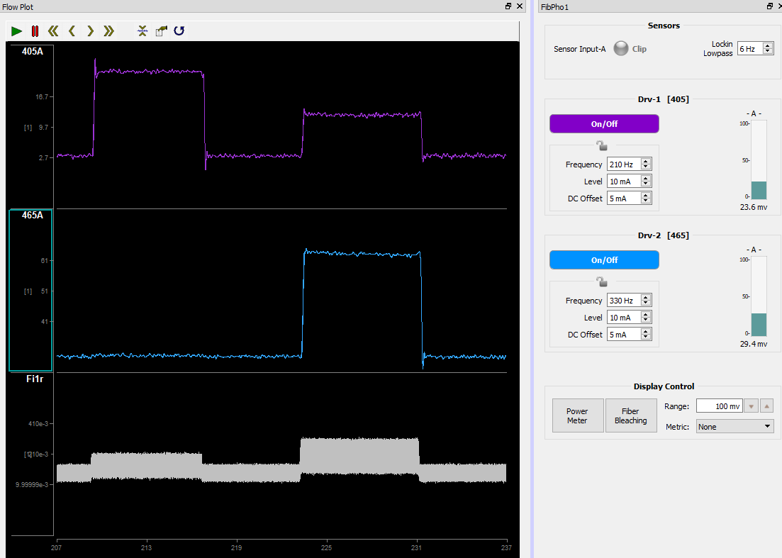
We also want to easily recognize which demodulated data stream we are observing by having them color-coded. Fiber Photometry experiments made in v94 or higher will have the demodulated streams colored based on excitation LED wavelength recognized in the Light Driver(s) 'Name'. You can change the color of data streams by double-clicking the y-axis of that stream Color Mode Set Color.

Note

You can rearrange or split out any flow plot stream into a new flow plot by selecting RT Layout or FP Setup and adjusting the window accordingly.

Note

These Run-Time images were taken with the 'Lock Freqs at Runtime' option off. This option is on by default and can be left on unless specific troubleshooting is needed.

Fiber Photometry Controls

The FibPho1 tab contains all the parameter controls for that gizmo (there would be multiple control tabs for each separate Fiber Photometry gizmo). The 'Sensors' and 'Drv-{N} [xxx]' sections have the same controls that were discussed in the Sensor(s) and Driver(s) tabs in The Fiber Photometry Gizmo chapter. There is an additional 'Display Control' section to toggle on/off Power Meter readings, set the system into Fiber Bleaching mode, adjust the range of the photosensor bar plot, and set a readout of signal distortion (Distortion), signal to noise (S/N), or nothing.

Note

The Power Meter and Fiber Bleaching options are only available during Preview Mode.

Sensors

The lowpass filter on the demodulated data can be changed in real time from 1-20 Hz by manually entering a value or adjusting the spinbox.

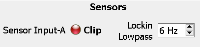
The Clipping Indicator for a respective sensor will illuminate red if the voltage levels of the analog photosensor signal exceed the clipping threshold set in the Sensor(s) tab in Design-Time. It will also illuminate if the input voltage is below 10 µV, which may indicate a bad connection.

Drv-{N} ['xxx']

Each light driver can be toggled On or Off by pressing the On/Off switch button. {N} is the driver number and ['xxx'] is the name assigned to that driver in Design-Time. The light drivers are on when the On/Off button is darkly colored; the button will be grayed out when drivers are off. There is an option for drivers on at runtime that can be enabled/disabled at Design-Time.

Frequency, Level, and DC Offset can be manually entered* or adjusted using the spinbox. Valid Frequency values range from 1 Hz - 5 kHz**. Valid Level and DC Offset values range from 0 mA - Max mA. The Max driver current is set during Design-Time.

Note

* The frequency values are locked at runtime by default. This is because, other than initial setup and debugging, the user likely should not change this value during a recording. You can unlock them by disabling the Lock Freqs at Runtime option in the Light Driver(s) tab at Design-Time.

Note

** Lock-in amplification works best when the driver frequency is high; the default values of 210 Hz, 330 Hz, etc. are good choices for the PS1 Lux photosensor, which has a low-pass filter corner at 700 Hz. Higher frequencies (1 kHz and above) can be used for specialized applications such as TEMPO (voltage sensor photometry) where sensors have a wider bandwidth. When running drivers at higher frequencies, however, make sure the acquisition processor rate (in the RZ gizmo) or the Required Sample Rate in the Fiber Photometry Gizmo is set high enough to avoid aliasing (at least double the driver frequency, e.g if you want to run a driver at 5 kHz you must set the acquisition processor rate to 12 kHz or preferably higher in Synapse).

The demodulated signal amplitude(s) for a Driver is shown as a bar graph display. There is one bar graph for each Driver x Sensor combination. The range of this bar graph can be adjusted in Display Control Range.

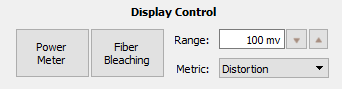
Display Control

The 'Power Meter' option will toggle readouts from a connected PM1. This is only available in Preview Mode. More on this in the Using the PM1 Power Meter section.

The 'Fiber Bleaching Option' will toggle the system into Fiber Bleaching mode. This is only available in Preview Mode. More on this in the Fiber Bleaching section.

Range sets the range on the photosensor bar graph in the Dvr-{N} [xxx] section.

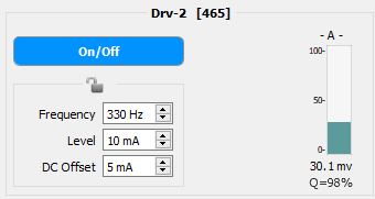
Metric can be set to 'None,' 'Distortion,' or 'S/N.' These numbers are displayed underneath the photosensor bar graph (see blue arrow).

Distortion measures the amount of signal distortion in the LED output signal relative to a pure sine wave at the set driver frequency. Distortion greatly impacts the demodulation measurement because it affects the frequency characteristics of the driving signal. While you generally want to keep the driving current low (to keep the overall light power low), you also want to make sure the distortion is also not too high. This measure is shown as a Quality-Score (Q-Score) on the runtime display and should ideally be >95%. A higher Q-Score is better. During system setup, adjust the Level and DC Offset settings to improve this value.

Adjusting LED Parameters (Level and DC Offset) - Using the PM1 Power Meter

The best way to setup your LED driver parameters, which includes the Level and DC Offset, is to use the Lux PM1 power meter. The PM1 can measure the power of multiple LED lights simultaneously and will inform the user about the Q-Score and transmission percentage* (Tx) of the LED signal through the optical chain.

Note

* The Launch Power Est option must be enabled in the Drivers tab in Design-Time to measure transmission percentage.

Important

Accurate power estimates require replicating the core diameters and NAs of your LED and Subject optical fiber cables as closely as possible. The LUX fiber kit includes 200 µm cables for the LED connections and a 400 µm cable for the PM1 measurements. If you are using 400 µm Subject cables with the LUX fiber kit, then your power estimate will be accurate. If you are using a 200 µm Subject cable, then your power will be up to four times higher than the power your Subject cable would provide.

If desired, you can use a 200 µm cable for the PM1 measurements. If you are using a 200 µm diameter Subject cable, then this should provide a more accurate power estimate. The 400 µm cable provided in the LUX fiber kit is low auto-fluorescence, so TDT recommends bleaching the 200 µm cable for at least 1 - 2 hours prior to measuring LED power.

To use the PM1, connect an FC - FC cable of the same diameter as your subject cable from the output of the subject fluorescent port (labelled 'Subject' on a Doric Minicube) directly to the input of the PM1. Because the core diameter is the same as your subject patch cable, this will effectively be the light power at the ferrule tip*. You can also measure the power at the tip of your real subject cable by placing the end partially into the PM1. The accuracy of this will vary based on how far in you place the cable end, but it will provide an idea of whether the cable can transmit the expected power you measured from the FC - FC cable earlier.

Note

* This is not the power at the implanted fiber optic tip. TDT recommends also measuring the power at the implant tip directly or calculating the transmission percentage of implants to estimate the light loss between the subject patch cable output and the implanted fiber tip.

'Power Meter' mode is available during Run-Time (Preview mode only). The PM1 can be accessed by both Lux I/O banks. This means that if your first bank is full of PS1 photosensors, then you can still use the PM1 on the second bank to measure LED power and cable transmission.

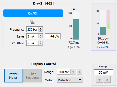
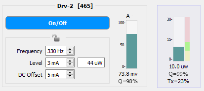
Enable the 'Power Meter' option in Display Control at Run-Time. This will display a new bar graph next to the photosensor readout for each LED driver. The bar graph and its associated 'Range' are highlighted here in this document in blue boxes.

As described in the Power Meter section, the green fill is 75% - 133% of your target power range. The green/blue bar is the measured power from the PM1.

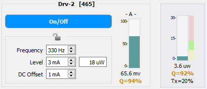
Below is a comparison of two PM1 readings of a 465 nm signal going through a 200 µm core diameter optical chain (except to the PS1, which is 600 µm core diameter). The target power is 10 µW per LED. In the first image, the Level and DC Offset have been adjusted to hit the target power and to maximize the Q-score in the Power Meter bar graph. In the second image, the DC Offset has been adjusted too low and the power is also outside of the target range. The too-low DC Offset decreased the Q-Score to 92%, which is too low to proceed with an experiment. Even if the Level was increased to hit the target power, the Q-score would likely still be too low, thus indicating that further adjustments (DC Offset up, Level down to meet the target) are needed.

Note

The Q factor on the PS1 bar graph (the left one closest to the Driver controls) and the clipping light should be ignored when measuring power from the PM1. The PM1 has fluorescent slides that will create a large return signal. This can often cause the PS1 to clip, which would, in turn, reduce the PS1 Q factor.

Also shown in the Power Meter bar graph is the Tx percentage. This indicated the amount of light transmission that goes through from the LED to the subject cable. This number is calculated based on the expected output (44 µW in the left image and 18 µW in the right image) versus the actual measured power.

Important

If applicable, all users should perform an initial PM1 setup prior to proceeding with in vivo experiments.

Benchtop Testing

If they are not already, please change the LED driver frequencies back to the defaults of 210 Hz and 330 Hz, or some other appropriate frequency. Lock-in amplification of the low-frequency fluorescent signals works best at high frequencies (200 - 530 Hz) with a wide frequency separation between driver frequencies. Make sure your driver frequencies are not multiples of one another and not a multiple of mains power (50 Hz or 60 Hz).

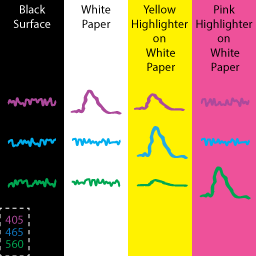
Our goal for this section is to demonstrate detection of fluorescent responses for each of our LED signals. To do this, we will need surfaces of different colors to serve as controls. The figure to the right depicts how LEDs of different colors would respond to Black, White, Yellow, and Pink surfaces. For our 405 nm and 465 nm setup, we will be using Black as a neutral control, white paper as a control for 405, and yellow highlighter as a control for both lights. Highlighter is a cheap solution for accomplishing this task. If more specific responses are desired, you can purchase fluorescent slides from Ted Pella.

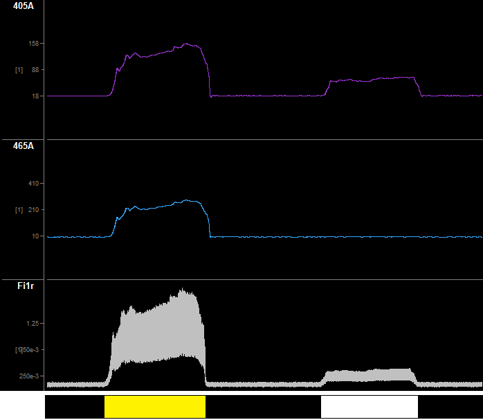
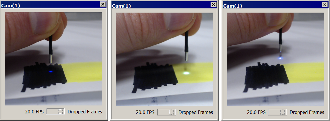
Shown in the Cam(1) images below is my in vitro setup for testing fluorescent demodulation. Both LEDs are on. To the right is a time-series of my response to each surface. Using a time span of 30 or 60 seconds is helpful for viewing (double click the x-axis on the bottom of the flow plots to change the time span). The black surface should have no significant fluorescence. As the cannula moves over the yellow highlighter surface, the amplitude of all signals increases because the fluorescence is non-specific but strong. When the cannula is over the white paper, only the 405 signal increases significantly.

Monitor your Fi1r signal and clipping indicator while doing this task. The demodulated signal will drop out if the light clips. This is because a clipped light is a DC signal, and thus there are no distinct sinusoidal characteristics to demodulate. If your photosensor is clipping, then try increasing the distance from your surfaces or decreasing the Level. If issues persist, see the Troubleshooting FAQ for more information.

In-vivo Testing

Once you have confirmed system functionality, you are ready to test on a prepped subject. The procedure for checking the Fi1r signal and adjusting parameters using the PM1 power meter is very similar to the benchtop method. The DC Offset you set in vitro should work in vivo. The Level you choose will depend on the desired light power and whether you see a response. If your light was very bright during in vitro testing, you will likely want to turn down the Levels as to prolong the risk of photobleaching.

With the cannula inserted into the implant sleeve, turn your LEDs on. Check the Q-Score (Display Control → Metric → Distortion) in the Drv bar graph (not the Power Meter bar graph) and make sure it is not yellow or red. Also make sure you are not clipping on the high-end or low-end and adjust the Level if your waveform is too large.

If the driver and Fi1r characteristics are okay, then adjust the time span to 30 seconds so you can better observe fluorophore activity.

Allow the signal and the subject to settle for a couple minutes. Ideally, there will not be downward drift in your demodulated data streams. If there is, then consider turning down the Level or photobleaching your cables before the next experiment. Once settled, perform either a startle (air puff, startle stimulus) or tail/foot pinch test, or another action that will invoke an expected response if those will not work, and observe the demodulated data streams.

Below is an example demodulated trace with GCaMP responses marked by black ticks. This has the iconic sharp rise at the onset of activity, then a slow decay back to baseline levels. There is also another example of a good GCaMP response trace in the Calculated Outputs section. GCaMP responses across experiment and observed cell group types may be different, and the amplitudes will vary by light intensity, targeting accuracy, cell count, animal age, and GCaMP expression levels. Note, this is the demodulated response curve and not dF/F, although the waveform shapes would look nearly identical if it was dF/F.

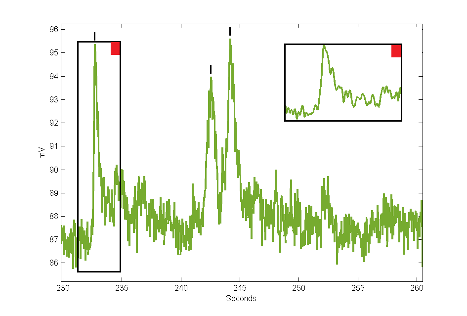Data from Workbook Example

Motion Artifact

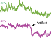
Motion artifact can occur during recordings. This shows up in the Fi1r and demodulated data streams as sudden changes in light and expression levels. The reason is because the cannula has shifted, so the cone of light, and thus the cone of fluorescent response, has changed. In order to detect motion artifacts, compare the isosbestic 405 nm stream to the 465 nm stream. If you see similar sudden changes in the continuity of the streams (level is not important as each stream will be different) in both streams, then there was likely a motion artifact. An example is to the right, where you can see a sharp drop in the 405 nm signal, and an overall baseline shift in both signals after the event. It is important to recognize motion artifacts because they may sometimes appear as promising GCaMP responses in the demodulated streams. If motion artifacts are occuring, then it may be because the subject cable is moving around inside the sleeve, the sleeve itself is too loose, or the implant is wiggling around inside the dental cement or brain itself (the brain naturally moves around the implant a little, but I mean that the fiber optic core is jostling around). You should also check for excessive cable bending, too, upstream of the animal. Make sure that the fiber optic cable connecting from the minicube/ mirror ports to the subject (or to rotary joint then to subject) are fairly straight and not too bent or twisted.

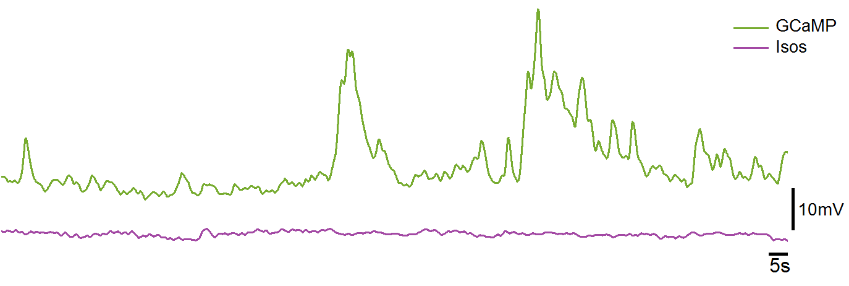
The ideal isosbestic control signal stays regular and flat during GCaMP activity, with only minor modulation that result from the demodulation process, as shown on the UV stream in the figure above. Data from Workbook Example

405 nm or 415 nm are widely used as isosbestic wavelengths for different types of GCaMP, as the total absorption of those wavelengths of UV light does not change during calcium activity changes (calcium independent measurement).

Note

In some cases of very large GCaMP activity, you may see an associated decrease in the 405 nm response signal. This is because 405 nm is slightly to the left of the true isosbestic point of GCaMP6 and newer, and calcium-unbound GCaMP can cause an associated dip in the control signal. This is rare, but can be advantageous for identifying biologically relevant signals online. However, if these events occur, you will have to be more careful in post-processing to not artificially increase event-related dF/F responses in your GCaMP trace via subtraction of the isosbestic control.

Easy First Targets and Controls

To verify system functionality in vivo, consider selecting easy areas that have GCaMP responses to simple stimuli (foot shock, tail pinch, reward), such as prefrontal cortex (PFC) or ventral tegmental area (VTA) or Barrel Cortex (stimuli is air puffs on whiskers), might be helpful for visualizing responses in subjects before approaching less characterized or harder to target populations.

Check with literature to see what standard controls are used to verify proper GCaMP activity. This often includes histochemical staining to confirm GCaMP expression within target cell types and sham recordings of animals without fluorophore expression during task trials.

If you are doing optogenetic stimulation, then performing controls is important to prove that the optogenetic light is not creating an artifact in the demodulated GCaMP data. This is because optogenetic stimulation wavelengths are close to those used in fiber photometry but are a much higher power, so there is a risk of light artifacts in the photosensor interfering with GCaMP data collection. A control could either be to stimulate in an animal without the opsin expression, but which has fluorophore expression, or to stimulate with the opsin expressed and record area without GCaMP expression. This is especially important if the opsin and fluorophore are in the same area and the light is being routed through the same fiber.

Fiber Bleaching

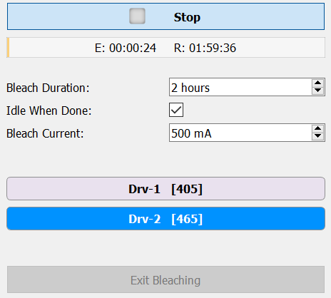
The fiber photometry gizmo has built in photobleaching controls (Display Control → Fiber Bleaching) to help users bleach their patch cables before recording.

TDT recommends that users photobleach at least their subject cables (it cannot hurt to bleach all cables) for ~1-2 hours at 500 mA prior to a subject recording to get the best signal to noise ratio (SNR). However, in practice, you can photobleach once a week with good results. Modern subject cables are 'low autofluoresence' to begin with and the levels of AF recover to baseline over a 1 - 2 week period after an effective photobleaching session.

The best to photobleach your subject cable is to attach it directly to the output of the LEDs that are being used in the experiment. Since this can only be one one at a time, you will need to photobleach for each wavelength. If you have a rotary joint, please also connect that in the photobleaching optical chain.

Important

Please make sure the cable is in a safe area where nobody can accidentally stare into the light output. Please refer to the LED Safety Information section for more details.

Important

Please turn off the RZ10x before adding or removing any optical cables from the banks of the RZ10x.

The photobleaching uses a constant current output to shine high light power through patch cables to reduce autofluorescence; 500 mA Bleach Current is recommended. The user can set the total duration, which LEDs are active, and the current output for the bleaching. Synapse will Idle and the LEDs will turn off when the timer finishes.

Note

The Fiber Bleaching option is only available during Preview Mode.

To read more about fiber auto fluorescence and photobleaching, please check the Doric or Thorlabs manufacturer websites. For Thorlabs, please see the 'Photobleaching' tab and the paragraph on photobleaching in the 'Overview.'

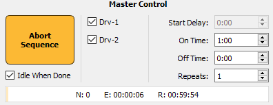
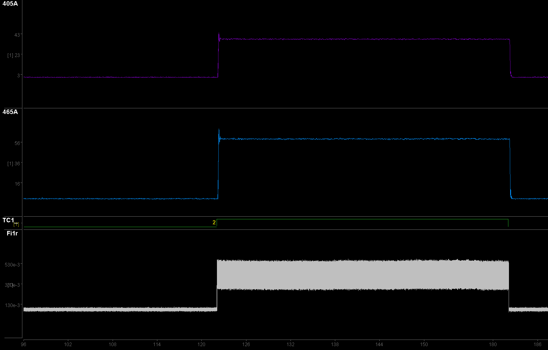
Timer Control

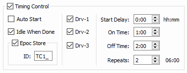
The Timing control options are used to cycle the LEDs On and Off for set durations and repeats during Run-Time.

This feature is very useful for researchers running long (greater than 1 hour) experiments where photobleaching becomes a concern.

The 'Idle When Done' option will return Synapse to Idle mode upon completion of the timing sequence.

The Epoc Store 'TC1_' will provide onset and offset timestamps for On Time and Off Time periods.

Run-Time recording notes

Run-Time recording notes are often very useful for marking when in vivo events, such as drug injections, occurred. These notes get saved as a text file in the data block. If Notes + Epocs is enabled, then a timestamp will also be added to the data. These epocs will be imported as a part of your data structure for later import.

Note

These should not take the place of programmatic timestamp markings of things like lever presses, foot shocks, lickometer events, etc. These more precisely-timed events are best implemented using the Digital I/O inputs (see Troubleshooting FAQ).

See this Lightning Video for an example.