OpenSorter Basics
This section introduces the various displays, tools, and sub-windows that make up the workspace.
The Workspace
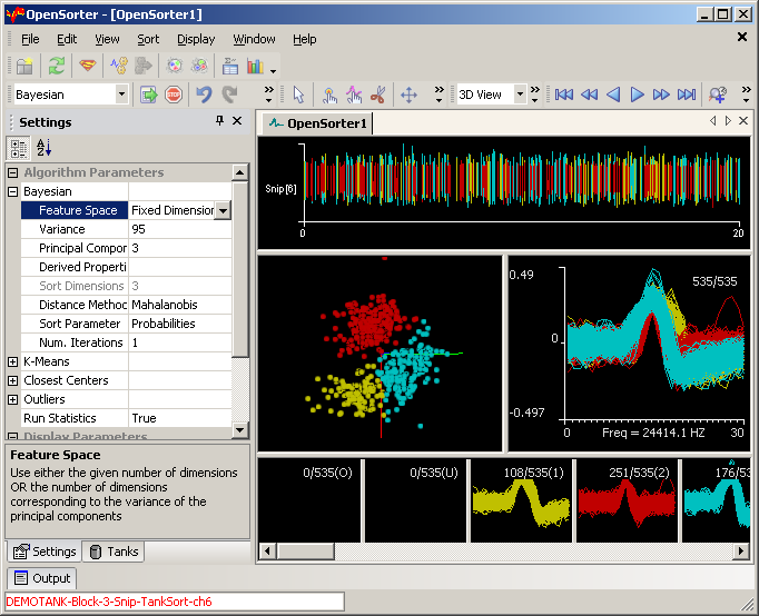
OpenSorter provides a versatile workspace where users can explore data sets and edit sort codes in a graphical environment. The customizable workspace includes collapsible panels that can be docked or floated and provides auto hide push pin tools to provide the most flexible workspace possible.
Tabbed Windows
The main workspace feature is a multi-pane tabbed window for displaying and editing data.
The window includes waveform space and feature space panes as well as a timeline pane and
individual unit waveform display. Multiple tabbed windows can be opened for viewing multiple
data sets. See Viewing Data in the Tabbed Window for
more information.
Menus and Toolbars
A comprehensive set of menus and toolbars provides easy access to commands and tools.
Frequently-used commands are available via toolbar buttons. Move the mouse pointer over a
toolbar button to display a tool tip that describes the function of that button. You can
move the toolbars and dock them to the top or bottom of the screen or rearrange and customize
the contents of the toolbars using the View | Toolbars sub-menu. See the
Menu and Toolbar Reference for a complete list of commands
and tools. Context sensitive menus are available by right-clicking the various panes of the
Tabbed Window.
Tanks Panel
A collapsible panel provides a convenient method of selecting data sets. Recently used
DataTanks are displayed for quick selection.
Tank Filtering Panel
A collapsible panel provides access to applying tank filter settings for event data.
Settings Panel
A collapsible panel provides access to property settings for each algorithm as well as
outlier methods, statistics, and feature space display properties. This window is described
in greater detail in the relevant sections.
Sort State Panel
A collapsible panel displays current algorithm, settings, and statistics.
Output Panel
Error messages are displayed in the Output panel.
Status Bar
A status bar along the bottom of the window identifies the current data set, SortID, and
channel.
Working with Panels, Panes, and Windows
OpenSorter makes use of tabbed windows, panes, and panels to organize the workspace. The flexible design allows the workspace to be reorganized or reconfigured quickly to meet work habits or particular tasks.
Panels
The collapsible panels organize task related features, such as selecting data and setting algorithm parameters. When not in use, they can be easily hidden, or minimized, to provide more space for displaying data or editing sort codes in the tabbed window.
To close a panel:
- Click the X in the top right corner of the panel.
To open a closed panel:
- Click the panel name on the View menu.
To hide a panel:
- Click the
 push pin in the top right corner of the
panel.
push pin in the top right corner of the
panel.
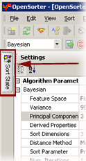
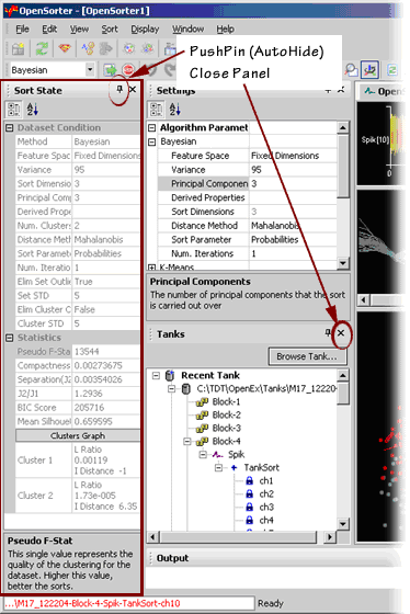
When a panel is hidden, it is represented by a tab-like button along the edge of the workspace.
To quickly show a hidden panel:
-
Point to the panel's button.
Note
The panel will be displayed, but will hide again when the pointer is moved away.
To unhide the panel:
-
Point to the panel's button. When the panel is displayed, click the push pin button to pin the panel to the workspace.
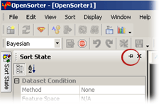
You can resize an open panel by dragging an edge of the panel that is adjacent to another sizeable area.
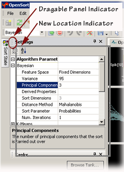
The gray dotted line along the left edge of the panel's title bar indicates that it can be dragged to a floating position or to a new position in the workspace. Floating panels can be positioned anywhere on the desktop, including areas outside the boundaries of the workspace.
To float or move a panel:
-
Click the title bar and drag it to a new location.
A gray box appears as the panel is moved indicating the new location.
To float the panel:
- Point to a location away from any edge of the window.
To move the panel to a new docked position:
- Point to a location along the edge of the workspace.
To create a tabbed panel:
-
Drag the panel over another panel until a tab shape appears along one edge.
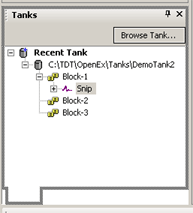
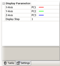
In a tabbed panel you can toggle between open panels by pointing to the tabs.
Windows and Panes
The tabbed window is the primary workspace. It is divided into several panes, to provide different views of the data for display and editing. Unlike the panels described above, these panes cannot be rearranged or hidden. All panes are in view whenever the window is open. However, the panes can be resized.
To resize a pane:
- Point to the splitter bar until a double sided arrow is displayed, then click and drag to resize the pane.
Multiple Tabbed Windows may be opened to view several data sets simultaneously. The tabbed window provides several different views of the data set. See Viewing Data in the Tabbed Window for more information.
Selecting a Data Set in the Tanks Panel
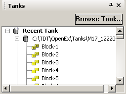
The Tanks panel is a collapsible panel that can be docked or floated depending on the user's needs. The panel displays DataTanks in a tree structure and allows the user to select the data set for display in the tabbed window.
Browsing For a Tank
If the desired DataTank is not in view, click the Browse Tank button in the Tanks panel, then select the desired tank in the Find Tank dialog box.
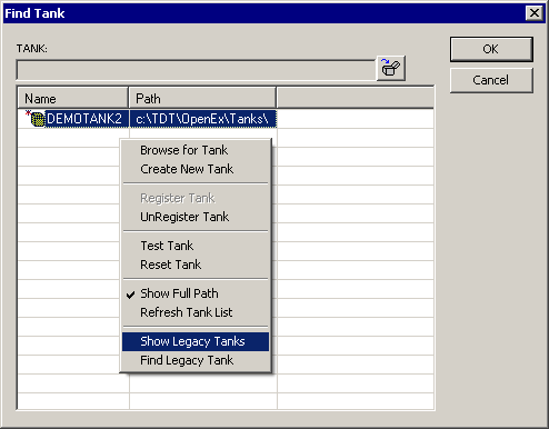
By default, the Find Tank dialog displays registered tanks in the current tank format. The shortcut menu (right-click) provides tools to locate additional tanks.
Show Legacy Tanks: view legacy tanks (tanks generated in versions prior to v2.0)
Browse for Tank: locate unregistered tanks in the current tank format
Find Legacy Tanks: locate unregistered legacy tanks
Note
Tanks can be registered or unregistered in the Find Tank dialog box at any time using Register Tank and UnRegister Tank on the shortcut menu. If a previously registered tank is deleted or moved without first being unregistered, the tank will still show up in the Tanks window.
Displaying Data for Sorting
To display a dataset in the tabbed window, expand the tree structure to reveal the desired data set then double-click to select it. The data is displayed in the tabbed window.
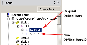
About the Tanks Panel Tree Structure
The DataTank structure can be thought of as hierarchical. Each DataTank might include multiple
blocks, each block might contain several spike events and each block might include several
channels. When viewed in OpenSorter, only snippet events are displayed. The original data is
displayed as it was acquired under a SortID called TankSort. Post hoc sorts are displayed with
a user specified SortID, such as tk32-07 above.
Navigating Using the Keyboard
If the Tanks window is the active window, the arrow keys can be used to move up/down in the
tree. The right arrow key expands the branches.
The Save Changes Prompt
By default, each time you navigate away from the active data set in the Tanks panel you will not be prompted to save any changes you have made. You can change this default behavior from the Tree Navigation command on the File menu to prompt you to save changes or save changes automatically.
If set to prompt, a save prompt will be displayed when you modify and attempt to navigate away from the original online sort data set (TankSort). If you select yes, a new branch is created in the tree structure to represent the new SortID and any sort results or applied tank filters are saved in a separate folder within the block folder. The original data set (TankSort) remains unaltered.
If you have been working with a user-defined SortID, and choose to save the changes, these will be saved over your existing work in that SortID. To avoid losing your earlier work, click Cancel and save your work from the File menu or using the Save SortID button.
Using the Settings Panel
The Settings panel is a collapsible panel that can be docked or floated depending on the user's needs. It includes parameters for sorting algorithms and display parameters. Tips about each parameter are displayed in the bottom section of the window when the parameter is selected.
Note
Options for some settings can be selected by double-clicking the desired setting box in the list. This will cycle through the choices one at a time. You can also manually enter the desired value(s) for the setting.
Algorithm Parameters - This section contains parameters for sorting algorithms, calculating outliers, and enabling statistical information. These parameters are applied each time a sorting algorithm is run. See Configuring Your Algorithm for more information on the settings in the Algorithm Parameters.
Important
If set to True, the outliers will be calculated and information about outliers defined manually or using the outlier buttons on the Standard toolbar will be discarded. See Eliminating Outliers for more information.
Display Parameters - This section contains parameters for controlling how data is displayed in the tabbed window. See Display Parameters for more information.
Viewing Data in the Tabbed Window
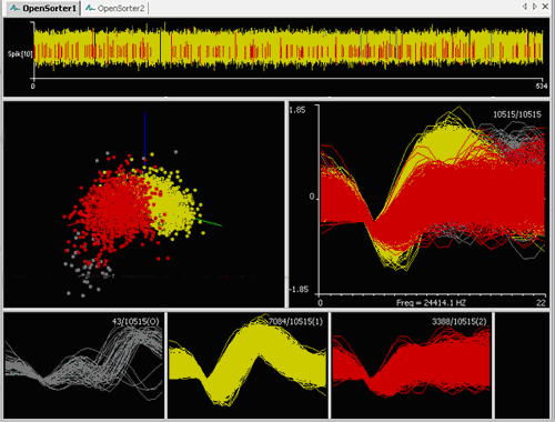
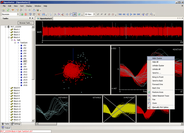
The selected data set is displayed in the tabbed window. Throughout all displays, each sort code (or "unit") is represented by a single color. Unsorted waveforms (U) are shown in light gray and outliers (O) are shown in dark gray. The Mouse toolbar provides tools to zoom, pan, or highlight data in any pane (see Mouse Toolbar). Clusters can be hidden, unhidden, or reordered from a short-cut menu (right-click) available in the Unit Display Pane (see below). Multiple Tabbed Windows may be opened to view several data sets simultaneously. The tabbed window provides several different views of the data set.
TimeLine Pane
A TimeLine pane runs along the top of the window to display spike waveforms across time. By
default, the entire time span of the dataset is displayed. Waveform amplitude is plotted on the
y-axis and time is plotted along the x-axis. The event label and channel number are also
displayed near the y-axis. If an individual trace has been selected using the mouse tools, a red
pointer is displayed below the x-axis to mark its position. The Navigation toolbar provides a
means of scrolling through the dataset and a Zoom TimeLine Region Tool can be used to examine
traces in a visually selected time span. See Navigating the TimeLine
for more information.
Waveform Space Pane
By default, the waveform space displays all spike waveforms in the data set. The waveforms are
aligned by sample number and colored by unit, or sort code. The number of waveforms in the data
set is displayed for easy reference. In this pane, users can manually classify waveforms based on
the actual waveform shape by drawing vertical/diagonal time-amplitude lines. All those spikes
that pass through the given range of amplitudes at times as specified by the line are assigned to
one sort code. See Using Manual Sort Methods for more
information on using the waveform space for manual spike sorting or refining sort results.
Feature Space Pane
In the feature space, waveforms can be viewed in terms of their pertinent properties, such as
amplitude or slope. This automatically reduces the dimensionality of the data while making it
visually easier to comprehend. By default, the feature space represents spikes in terms of their
first three principal components with PC1, PC2, and PC3 represented along the X, Y, and Z axes.
(The feature space used for sorting is actually calculated with as many principal components as
there are samples for each spike snippet and the display axes can be selected to be any of the first six
principal components.) Derived properties, such as the amplitude, slope and area of the spike
waveforms can also be computed and displayed in the Feature Space pane. Users can specify the axes
in the Settings panel under Display Parameters. This allows the user to explore and consider the
best combination of features to provide maximum cluster separation.
Unit Display Pane
The unit display pane provides a convenient means of viewing and comparing waveform shapes across
different units, or sort codes. A row of individual waveform plots displays the sorted waveforms by
unit; each individual plot displays all waveforms classified with a single sort code. Units are
displayed from left to right according to their numerical sort code.
When present in the data set, unsorted waveforms are assigned a sort code of "0" and will be displayed to the left of all other sort codes except outliers. Outlier waveforms are classified with a reserved sort code of "31" and will always be displayed in the first plot when present. If there are more units than can be displayed within the width of the tabbed window, a scroll bar is displayed. A numerical display in the top right corner indicates the number of waveforms displayed for the unit followed by the total number of waveforms in the data set. A sort code identifier is displayed in parentheses to the right of these numbers, with labels indicating the sort code number. An "O" or "U" in this field indicates outliers or unsorted waveforms, respectively.
The unit display pane supports all of the manual sorting tools and serves as an alternative waveform space in which to edit or refine sort results. A short-cut menu (right-click) provides menu options to hide, unhide, or reorder clusters in the other three panes. When a cluster is hidden an X is displayed across its subplot in the Units Display Pane.
Display Parameters
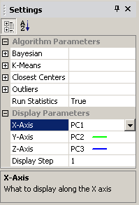
Parameters for controlling how data is displayed in the tabbed window can be found in the Settings panel. These settings only affect display. They do not affect the results of automatic sorting methods.
X-Axis: Select a derived property or principal component to be displayed as the x-axis in the feature space pane.
Y-Axis: Select a derived property or principal component to be displayed as the y-axis in the feature space pane.
Z-Axis: Select a derived property or principal component to be displayed as the z-axis in the feature space pane.
Display Step: Enter a value for n where every nth trace is displayed in the tabbed window panes. 1 to display all traces, 2 for every other trace, 3 for every third trace and so forth.
Tools for Viewing Data
The OpenSorter toolbars provide a variety of tools for viewing data. The Navigation toolbar and the Rotate toolbar group tools used in a specific pane of the tabbed window. The Mouse toolbar comprises a mix of viewing and sorting tools, most of which can be used in any pane. See Using Manual Sort Methods for more information on tools for fine tuning sort results or performing all sorting manually.
Each of these tools can be accessed via their respective menus or using the toolbar icons. A subset of tools specific to each pane can also be accessed by right-clicking in each of the panes.
To zoom or pan any pane:
- On the Mouse toolbar, click the button for the desired tool,
 Zoom or
  Pan, point to the desired pane then drag the
cursor across the pane.
Pan, point to the desired pane then drag the
cursor across the pane.
To reset a pane to its default settings:
- On the Mouse toolbar, click the
 Restore Default
Display button, point to the desired pane, then click the pane.
Restore Default
Display button, point to the desired pane, then click the pane.
To manually rotate the 3D view of the feature space:
- On the Mouse toolbar, click the
 Rotate 3D Display
button, click and drag in the Feature Space pane.
Rotate 3D Display
button, click and drag in the Feature Space pane.
To reset the mouse to the default state:
- On the Mouse toolbar, click the
 Default Pointer
button or right-click the display.
Default Pointer
button or right-click the display.
To highlight a trace in any pane:
- On the Mouse toolbar, click the
 Pick Nearest
Trace tool, then click the desired spike trace in any pane.
Pick Nearest
Trace tool, then click the desired spike trace in any pane.
The selected trace is highlighted in each of the display panes.
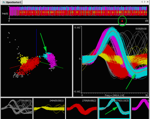
When a trace is selected a shortcut (right-click) menu is available and can be used to:
- Highlight the cluster (unit) to which the trace is assigned.
- Send the event (spike waveform) or cluster (unit) to another cluster (unit) or outlier group.
- De-select the event (spike waveform).
To reorder, hide, or unhide a cluster or clusters:
- Right-click the desired cluster in the Units Display Pane and select the desired option from the short-cut menu.
To view a selected time span in the TimeLine:
- On the Mouse toolbar, click the
 Zoom TimeLine
Region Tool and drag across the desired region of the TimeLine pane.
Zoom TimeLine
Region Tool and drag across the desired region of the TimeLine pane.
To navigate through the TimeLine:
- On the Navigation toolbar, click the desired button to move through the data incrementally.
Navigating the TimeLine
By default, the entire time span of the dataset is displayed in the TimeLine pane.

The Navigation toolbar provides tools for expanding or shrinking the displayed waveforms. Any manipulation of the timeline scale retains the earliest displayed time point in the display.


When the timeline is expanded, you can also move the timeline left or right to browse through the data (Duration refers to the visible width of the timeline pane).


To examine traces in a visually selected time span:
- Click the Zoom TimeLine Region Tool on the
Mouse toolbar and drag across the desired region of the timeline.


To reset the TimeLine to the default setting:
- Click the Restore Original Display button on the
Mouse toolbar then click the TimeLine pane.
Note that the timeline can be expanded or shifted such that no spikes are displayed at the current settings. The Restore Original Display, Move to Start or Move to End buttons are helpful to reconfigure the timeline to display useful data.
Viewing Large Datasets with Display Steps
By default, the entire dataset is displayed in the tabbed window. When working with large datasets it is sometimes helpful to view only a representative sample. In these cases, the user may choose to display every nth trace.
To view a representative sample of the data:
- Type the desired value for Display Step in the Display Parameters section of the Settings panel. Type 1 to display all traces, 2 for every other trace, 3 for every third trace and so forth.
Exploring Data in the Feature Space Pane
In the feature space pane, waveforms can be represented in terms of their principal components and/or derived waveform properties, such as the amplitude, slope, or area. By default, the feature space display is set for 3D viewing, but the interface provides a great deal of flexibility. You can rotate the display, select from several 2D views, or specify the axes to explore the best combination of features and viewpoints to provide maximum cluster separation. Users can use the mouse to define cluster centers (see Defining Centers) or to manually pick clusters (see Using Manual Sort Methods) in the Feature Space pane. Although the Feature Space can be displayed and manipulated in three-dimensional space, all points are mathematically transformed into the two dimensional display space for the purposes of manual sorting and editing. All mouse-based sorting tools operate in the two-dimensional display space.
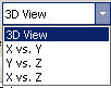
To select the 3D or 2D view mode:
-
On the Standard toolbar, click the View Angle box and select the desired view.
To manually rotate the 3D view of the feature space:
- On the Mouse toolbar, click the Rotate 3D Display button,
click and drag in the feature space pane.
The Rotate toolbar provides additional tools for rotating the data in the feature space, including tools to rotate along a specific axis or to start and stop automated, free rotation.
To reset a pane to its default settings:
- On the Mouse toolbar, click the Restore Original
Display button, point to the desired pane, then click the pane.
To specify any axis of the feature space display:
-
Expand the Display Parameters in the Settings panel.
-
Select the principal component or derived property from the drop-down menu adjacent to the axis to be changed. The axes in the Display Parameters menu are color-coded and match the three axes displayed in the feature space.