Plot Types

Selecting Data

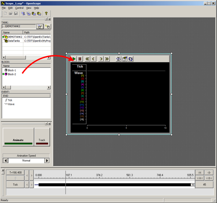
Before you can plot data, the tank and block within the tank must be selected in the Tank Select window of OpenScope.

To select data from a tank:

Click the tank name in the TANK area of the Tank Select window.
Click the block name in the BLOCK area of the Tank Select window. The events contained in the selected block will be displayed in the EVENT area.

Note

Most tanks created in Synapse do not show up in the Tank Select window until you have first browsed to them. You can add them to the registry to make them appear automatically.

After data is selected, plots can be created using the selected data.

Creating the Auto-Generated Flow Plot

The easiest way to quickly view data is using the basic Flow Plot.

To generate the Flow Plot:

Drag a Block from the Block list to the grid.

The Flow Plot is the same as the Synapse Flow Plot and contains the most common plot type for each Store in the data set.

Creating Pile Plots

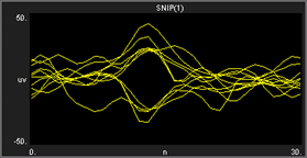
Pile plots are designed to visualize small data buffers (< 500) for quick recognition of differences in waveform properties. Pile plots are commonly used when extracellular recordings from neurons are examined to separate out single-unit activity. Users can use pile plots to view time stamped buffers, called snippets, or synchronized buffers. In a pile plot, the Y-axis is signal intensity such as voltage or dB and the X-axis is the record size in samples. Waveforms are layered over one another and centered along the X-axis. As the buffers pile up differences in the shape of the waveforms can easily be distinguished.

To quickly create a pile plot for a single channel of the selected data:

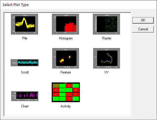
Drag a data event from the Tank select window to the grid area. The Select Plot Type box opens.
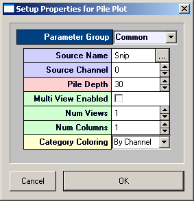
Click Pile. The pile plot is added to the grid area and the Setup Properties dialog box opens with the most commonly used settings for the pile plot displayed.
Related settings are grouped together by color. Other settings are available by clicking the Parameter Group box and selecting a settings group.
In the Source Channel box, enter the desired channel number.
In the Pile Depth box, enter the minimum number of wave forms to be displayed. The plot will be refreshed when the number of traces reaches twice the minimum.
Click OK.

The pile plot is configured for viewing a single channel of data. The plot can be positioned and resized using the mouse. When you animate or track data the plot will look similar to this:

After a single channel pile plot has been created, the settings can be quickly modified for multi-channel viewing.

To modify a pile plot to view multiple channels of data:

Double-click the plot to display the Setup Properties dialog box.
In the Source Channel box, enter 0 to ensure that all channels are available for viewing.
Select the Multi View Enabled check box.
In the Num Views box, enter the total number of views required to see all available channels of data in the multi view. This number will typically be the number of channels of data acquired. By default channels will be displayed beginning with channel 1.
In the Num Columns box, enter the number of columns to display.
Click OK.

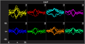
When you animate or track data the plot will look similar to this:

After a multi-channel pile plot has been created, the settings can be quickly modified for viewing a range of channels.

To modify a pile plot to view a range of channels:

Double-click the plot to display the Setup Properties dialog box.
Enter the total number of channels of data to be viewed in the Num Views box.
By default channels will be displayed beginning with channel 1. To display multiple channels beginning with another channel, modify the index offset.
To modify the index offset value, click the Parameter Group box, and click Multi View.
In the View Index Offset box, enter the number of channels to offset.

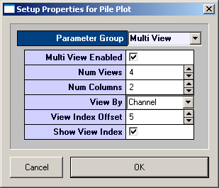
For example, to begin viewing from channel 6, enter an Index Offset value of 5. The plot will begin with channel 6 and display the next sequential channels to equal the number entered in the Num Views box.
Click OK.

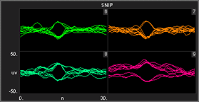
When you animate or track data the plot will look similar to this:

Creating Scroll Plots

Scroll plots provide a useful means of looking at continuous data. Data is presented in segments called scrolls. Looking at one scroll after another gives an effect similar to an oscilloscope or EKG. In a scroll plot the Y-axis is voltage and the X-axis is the record size.

To quickly create a scroll plot for single channel of the selected data:

Drag a data event from the Tank Select window to the grid area.

The Select Plot Type box opens.
Click Scroll
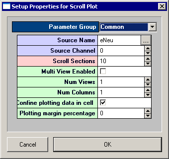
The scroll plot is added to the grid area and the Setup Properties dialog box opens with the most commonly used settings for the scroll plot displayed.
Related settings are grouped together by color. Other settings are available by clicking the Parameter Group box and selecting a settings group.
In the Source Channel box, enter the desired channel number.
Enter the desired number of scrolls, or data segments, to be displayed.
Click OK

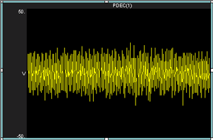
The scroll plot is configured for viewing a single channel. The plot can be positioned and resized using the mouse. When you animate or track data the plot will look something like this:

After a single channel scroll plot has been created, the settings can be quickly modified for multi-channel viewing.

To modify a scroll plot to view multiple channels of data:

Double-click the plot to display the Setup Properties dialog box.
In the Source Channel box, enter 0 to ensure that all channels are available for viewing.
Enter the desired number of scrolls, or data segments, to be displayed.
Select the Multi View Enabled check box.
In the Num Views box, enter the total number of views required to see all available channels of data in the multi view. This number will typically be the number of channels of data acquired. By default channels will be displayed beginning with channel 1.
In the Num Columns box, enter the number of columns to display. Leave this value set to 1 to see one channel per row.
Click OK.

After a multi-channel scroll plot has been created, the settings can be quickly modified for viewing a range of channels.

To modify a scroll plot to view a range of channels:

Double-click the plot to display the Setup Properties dialog box.
In the Num Views box, enter the total number of channels of data to be viewed. By default channels will be displayed beginning with channel 1. To display multiple channels beginning with another channel, modify the index offset.
To modify the index offset value, click the Parameter Group box, and click Multi View.
In the View Index Offset box, enter the number of channels to offset. For example, to begin viewing from channel 5, enter an Index Offset value of 4. The plot will begin with channel 5 and display the next sequential channels to equal the number entered in the Num Views box.
Click OK

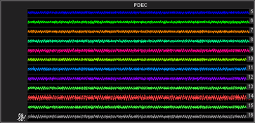
When you animate or track data the plot will look like similar to this:

Creating Histograms

Histograms use time stamped values from a variety of data Stores for graphic presentation. The most common of these are snippets, but lists and even scalars can be included as long as a time stamp is part of the acquired value. Users set up the bin size (size of time divisions for sorting the time stamps) and the parameters for refreshing the plot.

A common plot in neurophysiology is the peristimulus histogram, or PSTH. This plot shows the distribution of spike times after a stimulus has been presented. Another plot might show spike times for a particular epoch event such as a signal of particular intensity and a final plot might compare spike patterns across channels over the entire experiment.

Histogram plots in OpenScope show the distribution of waveform time stamps over a set time span. Histogram plots can show additive changes over a set time scale or they can be refreshed over a set range. In addition, the plots can refresh (start from zero) at each epoch or on changes in an epoch (such as a change in the intensity of a stimulus).

This view provides a good visual representation of how waveform time stamps are distributed from the start of a stimulus.

To quickly create a histogram plot of for a single channel of the selected data:

Drag a data event from the Tank Select window to the grid area. The Select Plot Type box opens.
Click Histogram

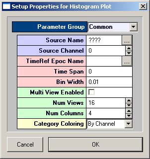
The histogram plot is added to the grid area and the Setup Properties dialog box opens with the most commonly used settings for the histogram plot displayed.
Related settings are grouped together by color. Other settings are available by clicking the Parameter Group box and selecting a settings group.
In the Source Channel box, enter the desired channel number. Channel selection is affected by the Index value on the Devices page and by the Store Chan Offset value on the Stores page.
In the TimeRef Epoc Name box, select an epoch, or indexed, event. This must be selected to update the histogram.
In the Time Span box, enter the desired time span. This might be set to the length of a stimulus, for example. In the Time Span box the time span can be fixed by the user or left set to 0 to respect the TRef duration. If the epoch is a stimulus this will allow you to see how waveform times are distributed from the start of the stimulus.
In the Bin Width box, enter the bin width. The bin width should relate to the distribution pattern of the time stamped signals. For a PSTH this might mean that the bin width should be a couple of milliseconds, for patterns of evoked potentials it could be much larger.
Click OK

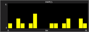
The histogram plot is configured for viewing a single channel. The plot can be positioned and resized using the mouse. When you animate or track data the plot will look similar to this:

After a single channel histogram plot has been created, the settings can be quickly modified for multi-channel viewing.

To modify a histogram plot to view multiple channels of data:

Double-click the plot to display the Setup Properties dialog box.
Enter 0 in the Source Channel box to ensure that all channels are available for viewing.
Select the Multi View Enabled check box.
In the Num Views box, enter the total number of views required to see all available channels of data in the multi view. This number will typically be the number of channels of data acquired. By default channels will be displayed beginning with channel 1.
In the Num Columns box, enter the number of columns to display. Depending on the design of your experiment you might want to view a pattern that is representative of the physical or logical distribution of the channels. For example, if you had electrodes placed in a 4 x 4 grid around the head then it would be useful to see that pattern in OpenScope. Similarly, if you had electrodes in a linear pattern you might want to have either 1 column or 16 columns.
Click OK

When you animate or track data the plot will look similar to this:

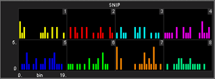
After a multi-channel histogram plot has been created, the settings can be quickly modified for viewing a range of channels.

To modify a histogram plot to view a range of channels:

Double-click the plot to display the Setup Properties dialog box.
In the Num Views box, enter the total number of channels of data to be viewed. By default channels will be displayed beginning with channel 1. To display multiple channels beginning with another channel, modify the index offset.
To modify the index offset value, click the Parameter Group box, and click Multi View.
In the View Index Offset box, enter the number of channels to offset.

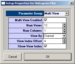
For example, to begin viewing from channel 5, enter an Index Offset value of 4. The plot will begin with channel 5 and display the next sequential channels to equal the number entered in the Num Views box.
Click OK

After a multi-channel histogram plot has been created, the settings can be quickly modified to view by sort code.

To modify a multi-channel histogram plot to view by sort code:

Double-click the plot to display the Setup Properties dialog box.
Click the Parameter Group box, and click Multi View.
In the View By box, select Sort Code from the drop down list.
Update the Num Views and View Index Offset values as needed.
Click OK

Creating Raster Plots

Raster plots provide a useful means of looking at time stamped values or waveforms that are not continuous, such as snippets. The time stamps of the snippets are represented by dots plotted in rows. Each row represents an epoch, or indexed, event. In a raster plot the Y-axis is indexed event values and the X-axis is time stamp values.

This view provides a good visual representation of when snippets occurred for an indexed event. Raster plots are an excellent way of detecting subtle changes in the timing of waveforms across channels.

To quickly create a raster plot for a single channel of the selected data:

Drag a data event from the Tank Select window to the grid area.

The Select Plot Type box opens.
Click Raster
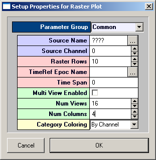
The raster plot is added to the grid area and the Setup Properties dialog box opens with the most commonly used settings for the raster plot displayed.
Related settings are grouped together by color. Other settings are available by clicking the Parameter Group box and selecting a settings group.
In the Source Channel box, enter the desired channel number.
In the Raster Rows box, enter the desired number of rows to be displayed.
In the TimeRef Epoc Name box, select an epoch, or indexed, event. This will define the Y-Axis.
In the Time Span box, enter a time stamp value for the maximum value of the X-axis. This value should usually be the time span of the indexed event, according to the time stamp.
Click OK

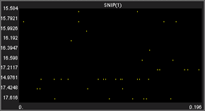
The raster plot is configured for viewing a single channel. The plot can be positioned and resized using the mouse. When you animate or track data the plot will look like this:

To modify a raster plot to view multiple channels of data:

Double-click the plot to display the Setup Properties dialog box.
In the Source Channel box, enter 0 to ensure that all channels ar available for viewing.
In the Raster Rows box, enter the desired number of rows to be displayed. Enter 1 to view one row per channel for a clear comparison across channels for a single event value.
Select the Multi View Enabled check box.
In the Num Views box, enter the total number of views required to see all available channels of data in the multi view. This number will typically be the number of channels of data acquired. By default channels will be displayed beginning with channel 1.
In the Num Columns box, enter the number of columns to display.
Click OK

To modify a raster plot to view a range of channels:

Double-click the plot to display the Setup Plot dialog box.
In the Num Views box, enter the total number of channels of data to be viewed.
By default channels will be displayed beginning with channel 1. To display multiple channels beginning with another channel, modify the index offset.
To modify the index offset value, click the Parameter Group box, and click Multi View.
In the View Index Offset box, enter the number of channels to offset.
For example, to begin viewing from channel 5, enter an Index Offset value of 4. The plot will begin with channel 5 and display the next sequential channels to equal the number entered in the Num Views box.
Click OK

To modify a multi-channel raster plot to view by sort code:

Double-click the plot to display the Setup Properties dialog box.
Click the Parameter Group box, and click Multi View.
In the View By box, select Sort Code from the drop down list.
Update the Num Views and View Index Offset values as needed.
Click OK

Creating XY Plots

XY plots provide a useful means of looking changes in two continuously varying values. In OpenScope, the Y-axis and the X-axis are selected from available data events. The XY plot can be used to plot positional information such as XY coordinates for an animal moving in a tank or it can be used to plot data from an eye or head tracker.

This type of plot can also be used when the study subject needs to be in a specific position for accurate data acquisition. The XY plot can help the user to quickly determine if there were any significant changes in the subject's position such as the head position relative to the position of a sound or visual stimulus.

To quickly create an XY plot for a single channel of the selected data:

Drag a data event from the Tank Select window to the grid area.

The Select Plot Type box opens.
Click XY

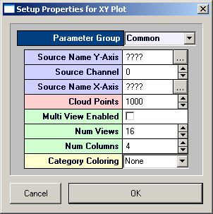
The XY plot is added to the grid area and the Setup Properties dialog box opens with the most commonly used settings for the feature plot displayed.
Related settings are grouped together by color. Other settings are available by clicking the Parameter Group box and selecting a settings group.
In the Source Channel box, enter the desired channel number.
Click the Source Name X-Axis box to select the desired data event for the X-axis. An event selection box opens.
Click the desired data event to select it, and click OK.
In the Cloud Points box, enter the minimum number of points to be displayed. The plot will refresh when the plot reaches twice the value set.
Click OK

The XY plot is configured for viewing a single channel of data. The plot can be positioned and resized using the mouse.

After a single channel XY plot has been created, the settings can be quickly modified for multi-channel viewing.

To modify a XY plot to view multiple channels of data:

Double-click the plot to display the Setup Properties dialog box.
In the Source Channel box, enter 0 to ensure that all channels are available for viewing.
Select the Multi View Enabled check box.
In the Num Views box, enter the total number of channels of data to be viewed.
By default channels will be displayed beginning with channel 1.To display multiple channels beginning with another channel, modify the index offset.
To modify the index offset value, click the Parameter Group value box, and click Multi View.
In the View Index Offset box, enter the number of channels to offset.
For example, to begin viewing from channel 5, enter an Index Offset value of 4. The plot will begin with channel 5 and display the next sequential channels to equal the number entered in the Num Views box.
Click OK

Creating Feature Plots

Feature plots compare two waveform properties, such as the first and second peak voltages of two candidate spikes. They are ideal for determining how many unique waveforms are present in a signal.

In OpenScope the feature plot has been designed for examining patterns of spike waveforms. The plot works best when viewing time stamped waveforms that are not continuous. In OpenEx this type of data is also called snippet data. Although other waveforms can be viewed, plotting complex waveforms with many points will require intensive amounts of computer time.

While the default feature of the Y-axis is the voltage of the second peak and the X-axis is the voltage of the first peak, the X-axis and Y-axis features can be selected from a drop down list in the Setup Properties dialog box. By generating multiple feature plots, each with different XY characteristics, it is possible to differentiate several spike types. This information can then be used to do offline or online spike sorting.

To quickly create a feature plot for a single channel of the selected data:

Drag a data event from the Tank Select window to the grid area.

The Select Plot Type box opens.
Click Feature

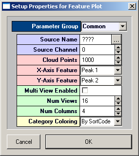
The feature plot is added to the grid area and the Setup Properties dialog box opens with the most commonly used settings for the feature plot displayed.
Related settings are grouped together by color. Other settings are available by clicking the Parameter Group box and selecting a settings group.
In the Source Channel box, enter the desired channel number.
In the Cloud Points box, enter the minimum number of points to be displayed. The plot will refresh when the plot reaches twice the value set.
If desired, select an X-axis and/or Y-axis feature from the drop down menus in the corresponding value box. Select from Total Amplitude, Peak 1, Peak 2, Peak to Peak Time, or Area.
By default, Category Coloring is set to By SortCode and a different color will automatically be assigned to each sort code. When data is not associated with a sort code it will be assigned a gray color. If sort codes are not present in the data, change this setting to None to display data points in a brighter color for easier viewing.
Click OK

The feature plot is configured for viewing a single channel of data. The plot can be positioned and resized using the mouse.

After a single channel feature plot has been created, the settings can be quickly modified for multi-channel viewing.

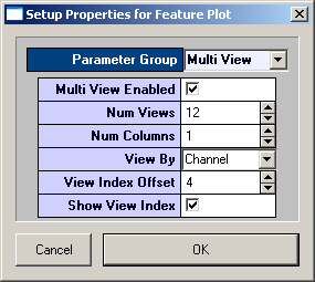
To modify a feature plot to view multiple channels of data:

Double-click the plot to display the Setup Properties dialog box.
In the Source Channel box, enter 0 to ensure that all channels are available for viewing.
Select the Multi View Enabled check box.
In the Num Views box, enter the total number of views required to see all available channels of data in the multi view. This number will typically be the number of channels of data acquired. By default channels will be displayed beginning with channel 1.
In the Num Columns box, enter the number of columns to display.
By default, Category Coloring is set to By SortCode and a different color will automatically be assigned to each sort code. When data is not associated with a sort code it will be assigned a gray color. If sort codes are not present in the data, change this setting to By Channel to display data points in brighter colors for easier viewing.
Click OK

After a multi-channel feature plot has been created, the settings can be quickly modified for viewing a range of channels.

To modify a scroll plot to view a range of channels:

Double-click the plot to display the Setup Properties dialog box.
In the Num Views box, enter the total number of channels of data to be viewed. By default channels will be displayed beginning with channel 1.To display multiple channels beginning with another channel, modify the index offset.
To modify the index offset value, click the Parameter Group value box, and click Multi View.
In the View Index Offset box, enter the number of channels to offset.

For example, to begin viewing from channel 5, enter an Index Offset value of 4. The plot will begin with channel 5 and display the next sequential channels to equal the number entered in the Num Views box.
Click OK

Creating Chart Plots

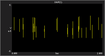
Chart plots are an excellent way of graphing time stamped waveform data such as spike snippets. Unlike raster plots that only show the position of the time stamp over a narrow range in the block, the chart plot shows the snippet waveform and its exact position in the block of data.

In a chart plot the Y-axis is voltage and the X-axis is time in seconds. When the scale of the X-axis is contracted the position of a snippet along the X-axis clearly identifies when in time the snippets occurred and patterns of occurrence over time are emphasized. As the scale of the X-axis is expanded the shape of the waveform becomes more visible.

To quickly create a chart plot for single channel of the selected data:

Drag a data event from the Tank Select window to the grid area.

The Select Plot Type box opens.
Click Chart

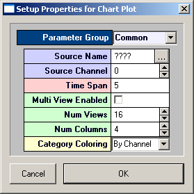
The chart plot is added to the grid area and the Setup Properties dialog box opens with the most commonly used settings for the chart plot displayed.
Related settings are grouped together by color. Other settings are available by clicking the Parameter Group box and selecting a settings group.
In the Source Channel box, enter the desired channel number.
Enter the desired Time Span in seconds, to be displayed on the X-axis.
Click OK

The chart plot is configured for viewing a single channel. The plot can be positioned and resized using the mouse. When you animate or track data the plot will look like this:

To quickly expand the X-axis scale and view a snippet waveform, hold down the SHIFT key, point to the snippet, and drag to the right.

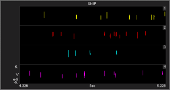
After a single channel chart plot has been created, the settings can be quickly modified for multi-channel viewing.

To modify a chart plot to view multiple channels of data:

Double-click the plot to display the Setup Properties dialog box.
In the Source Channel box, enter 0 to ensure that all channels are available for viewing.
Enter the desired Time Span in second, to be displayed on the X-axis. Selecting a shorter time span will improve animation performance for multiple channels. When viewing the chart, the time span can be shortened or expanded by pressing and holding the SHIFT key, and dragging right or left with the mouse.
Select the Multi View Enabled check box.
In the Num Views box, enter the total number of views required to see all available channels of data in the multi view. This number will typically be the number of channels of data acquired. By default channels will be displayed beginning with channel 1.
In the Num Columns box, enter the number of columns to display. Leave this value set to 1 to see one channel per row.
Click OK

When you animate or track data the plot will look like similar to this:

After a multi-channel chart plot has been created, the settings can be quickly modified for viewing a range of channels.

To modify a chart plot to view a range of channels:

Double-click the plot to display the Setup Properties dialog box.
In the Num Views box, enter the total number of channels of data to be viewed.
By default channels will be displayed beginning with channel 1. To displa multiple channels beginning with another channel, modify the index offset. To modify the index offset value, click the Parameter Group box, and click Multi View.
In the View Index Offset box, enter the number of channels to offset. For example, to begin viewing from channel 5, enter an Index Offset value of 4. The plot will begin with channel 5 and display the next sequential channels to equal the number entered in the Num Views box.
Click OK

Creating Activity Plots

Activity plots are used to view the amount of spike (or other) activity occurring on a given channel or group of channels. Activity plots make it easy to view spike counts or to compare spike rates between acquisition channels. Activity plots use time stamped values from a variety of data Stores for graphic presentation. The most common of these are snippets, but lists and even buffers can be included as long as a time stamp is part of the acquired value. Users define the minimum and maximum value to be displayed, assign a color to minimum and maximum, and choose a parameter for refreshing the plot. As the plot is animated the color of an activity cell varies in intensity across a range corresponding to the minimum and maximum defined values.

To quickly create an activity plot for combined data for all channels of the selected data:

Drag a data event from the Tank Select window to the grid area.

The Select Plot Type box opens.
Click Activity

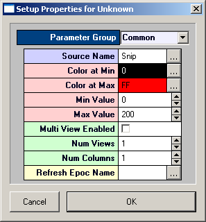
The activity plot is added to the grid area and the Setup Properties dialog box opens with the most commonly used settings for the activity plot displayed.
Related settings are grouped together by color. Other settings are available by clicking the Parameter Group box and selecting a settings group.
In the Refresh Epoch Name box, select an epoch, or indexed, event. This must be selected to update the plot.
In the Max Value box enter a number at least as large as the maximum activity (number of spikes) anticipated.
Click OK

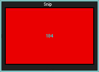
The Activity plot is configured for viewing combined data for all channels. The plot can be positioned and resized using the mouse. When you animate or track data the plot will look similar to this:

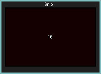Combined Data Activity Plot with Activity Near Minimum Value

Combined Data Activity Plot with Activity Near Maximum Value

After a combined data activity plot has been created, the settings can be quickly modified for multi-channel viewing.

To modify an activity plot to view multiple channels of data:

Double-click the plot to display the Setup Properties dialog box.
Select the Multi View Enabled check box.
In the Num Views box, enter the total number of views required to see all available channels of data in the multi view. This number will typically be the number of channels of data acquired. By default channels will be displayed beginning with channel 1.
In the Num Columns box, enter the number of columns to display. Depending on the design of your experiment you might want to view a pattern that is representative of the physical or logical distribution of the channels. For example, if you had electrodes placed in a 4 x 4 grid around the head then it would be useful to see that pattern in OpenScope. Similarly, if you had electrodes in a linear pattern you might want to have either 1 column or 16 columns.
Click OK

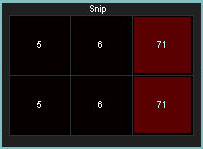
When you animate or track data the plot will look similar to this:

After a multi-channel activity plot has been created, settings can be modified to view by sort code.

To modify a multi-channel activity plot to view by sort code:

Double-click the plot to display the Setup Properties dialog box.
Click the Parameter Group box, and click Multi View.
In the View By box, select Sort Code from the drop down list.
Update the Num Views and View Index Offset values as needed.
Click OK